Core Concepts
This section contains background of concepts that are common across all of HEBI’s hardware and software products. As much as possible, information here is presented in a general form while more hardware-specifc or language-specific details are provided, respectively, in the Hardware and Tools/APIs sections.
Modules
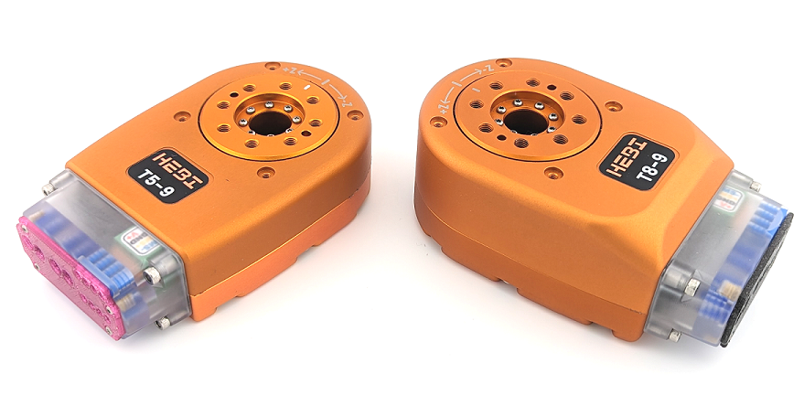
HEBI modules are Ethernet-enabled devices that serve as building blocks for a robot or automated system. These modules include actuators to provide physical motion, and devices to interface with other sensors and I/O. Modules run firmware that allow them to communicate over a standard Ethernet connection. Aspects of the firmware that are common to all modules are documented below, while aspects that are module-specific are covered in the in the Hardware section.
Communications
Modules are connected to host computers via standard Ethernet and standard commercially available networking equipment. In an Ethernet network every client needs to obtain an IP address in order to communicate. There are two ways to get an IP address:
Dynamic Address Assignment (DHCP)
| For most situations, we recommend that you use dynamic address assignment (DHCP). This requires you to connect your computer and the modules into a network with router that supports DHCP. New modules ship configured for DHCP by default. |
| If your network does not already have a router we recommend that you purchase a router. In some cases your network enforces security policies that do not allow unregistered devices on the network, or your computer may also have its network settings restricted or firewalled. Please work with your IT department to resolve these issues. |
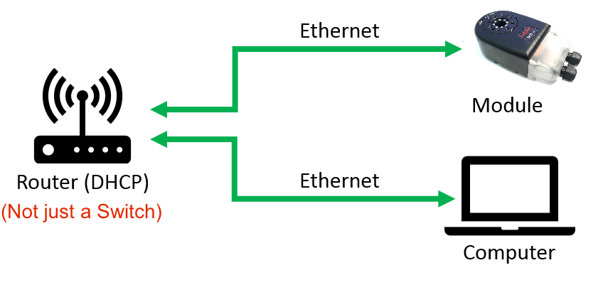
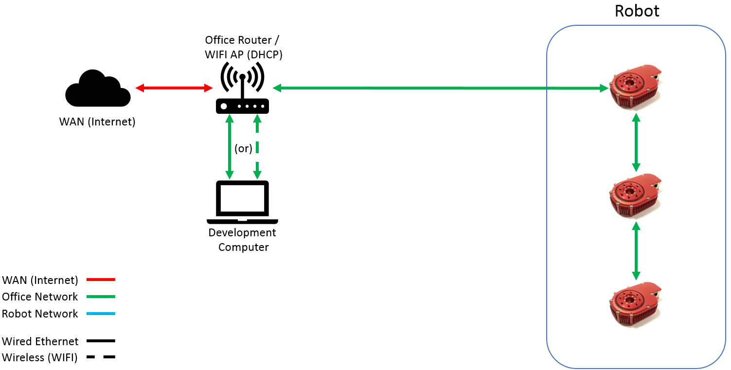
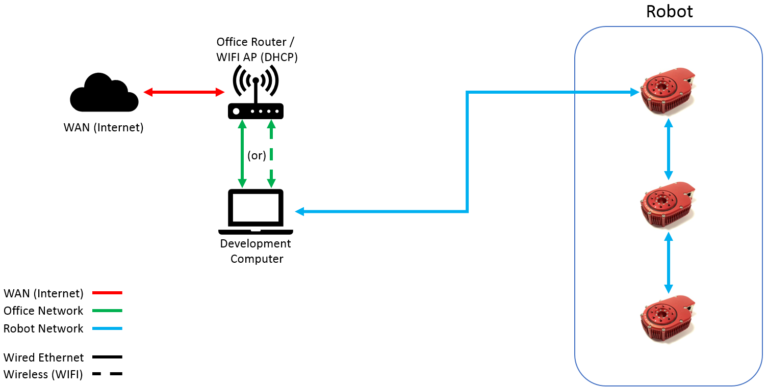
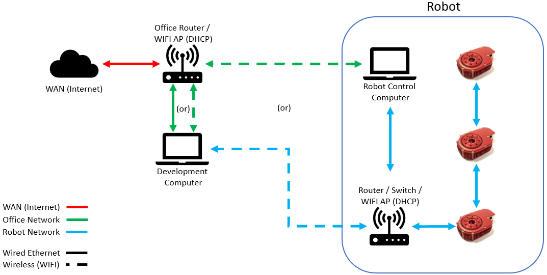
The image above shows the basic network configuration for communicating with HEBI actuator. The computer and the actuators are both connected to a router. Virtually all consumer-grade routers have DHCP enabled by default, so a quick search on your shop of choice (e.g. Amazon) for Ethernet router should work. Some examples are listed below:
Getting Started
-
Plug the computer as well as your module(s) into the same router as shown above. You can daisy-chain multiple modules or extend the network using an Ethernet switch.
-
Power on the modules and look at the LED color. Blinking orange/green means that it is searching for an IP address. Once it turns into a green fade, the modules has obtained an IP address.
-
You can check whether communications have been setup correctly by running the Scope GUI or any of our APIs.
Static Address Assignment
| We recomend setting up a static IP network only if you have a strong understanding of IP configuration. For more information on manually configuring a network, please refer to Understanding TCP/IP addressing and subnetting basics. |
IP addresses on each module can be set statically so that they don’t need to query for an address every time. This can be useful when:
-
It is difficult to integrate a router or DHCP server
-
The robot needs to interface with other equipment on static network
-
The robot needs to initialize instantly on power-up
Static IP addresses can be set by right-clicking on a module’s entry in the Scope GUI as highlighted below.
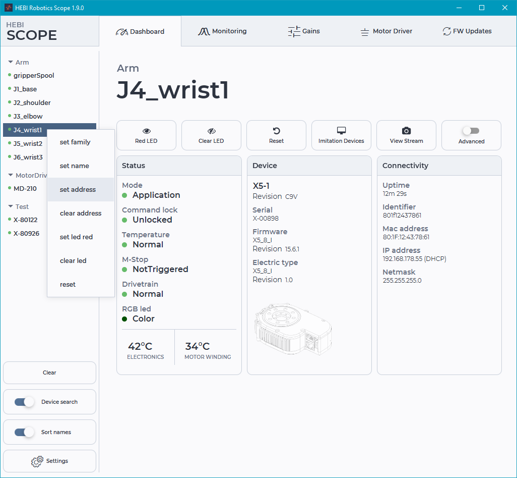
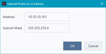
This will open the following dialog that allows for setting the IP address and subnet mask. The values default to the device’s current address and subnet mask. Settings will take effect after the module is restarted.
|
When setting static IP addresses it is important to manually keep track of what addresses have been assigned. Every device on the network needs to have a unique IP address. If two or more devices (modules, host computers, or any other device) have the same address the network may not work. Additionally, it is important that the subnet mask be set to the same value across all devices. For almost all applications we recommend keeping the default subnet mask of |
Connectionless Static IP Reset
| Connectionless static IP reset is only supported on firmware versions 15.0.0 and newer. To update your modules to the latest firmware, click the "Firmware Updates" tab in Scope. |
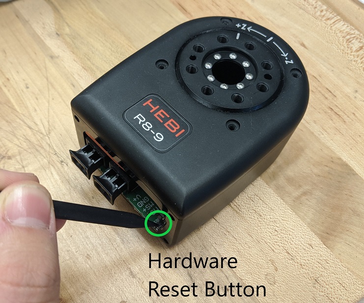
You will be unable to connect with a module if it is set to DHCP and you do not have a router on hand or if the module is set to an unknown static IP address. To recover access to the module in these circumstances, the module can be reset to a known default static IP address using the following procedure:
-
Power on the module.The LED should start fading green or blinking orange/green.
-
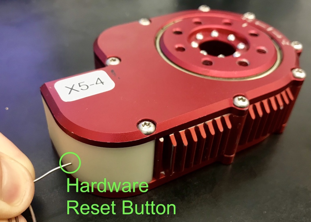
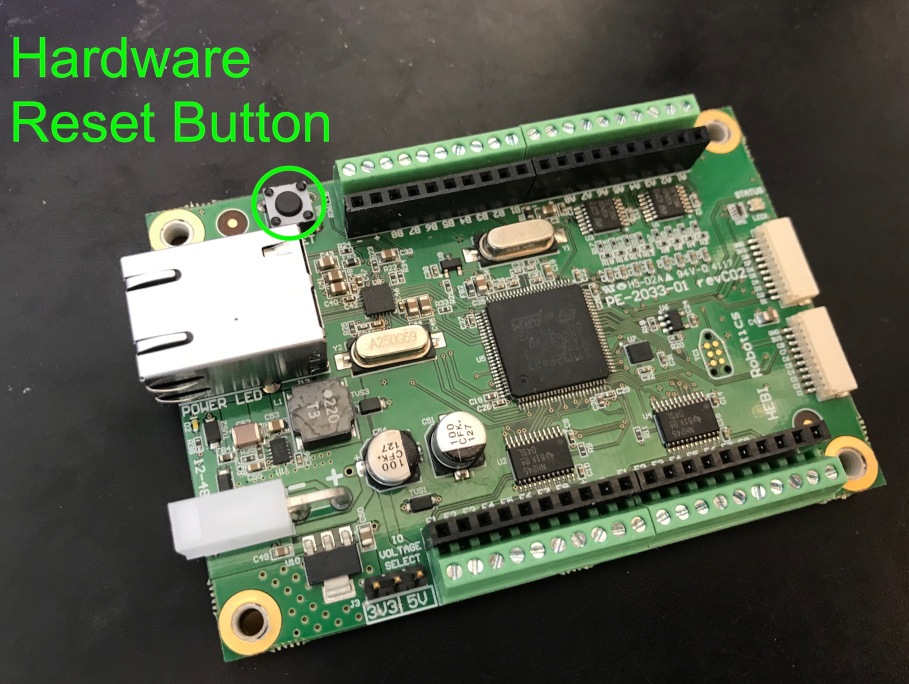
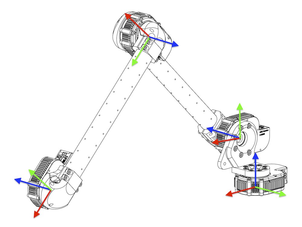
Press and hold the hardware reset button (images above). On X-Series actuators, you will need to use a paper clip to press the button inside the connector cover (see images above).
-
Continue holding until the LED changes to a fast green flash and let go of the reset button.
-
The module will reset and have the static IP address
10.11.12.13with subnet mask255.255.255.0. -
To connect to the module your computer will have to have the subnet mask set to
255.255.255.0and the IP address set to10.11.12.XXX, whereXXXis not13or the address of any other device on the network.
Resetting Module back to DHCP
Modules can be set back to DHCP by right-clicking on the module in Scope and selecting "clear address" in the same menu as "set address".
If the module is not accessible in Scope (e.g. you don’t know its static IP address) you can also revert to DCHP by doing a hardware reset using the following procedure:
-
Make sure the module is powered off.
-
Press the hardware reset button (images above). On X-Series actuators, you will need to use a paper clip to press the button inside the connector cover (see images above).
-
Power on the module. The LED should start fading red.
-
Wait until the LED does a faster-blink red and let go of the reset button.
-
Power the module off, and then power it back on again
Connections to Multiple Networks
Control computers may have more than one network interfaces and be connected to more than one network. For example, computers can be on wired Ethernet and WiFi at the same time. In order to find modules on all networks, the default behavior for the HEBI module lookup is to broadcast on all interfaces.
| Note that in some applications and APIs the local networks may be determined only once on startup, so changing your network, e.g., plugging your computer into a different router, may require a refresh or restart of the app/API. |
Example Robot / Network Configurations
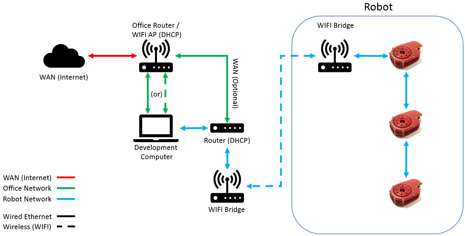
There a number of different ways you can configure the network between the computers and the modules, depending on the needs of your application. Below are a number of different setups that we have made for various robots.
| To view a larger version of the diagrams below, right-click the image and open in a new tab. |
| Summary / Description | Diagram |
|---|---|
Office Network w/ DHCP |
|
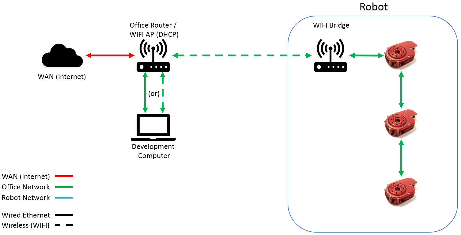
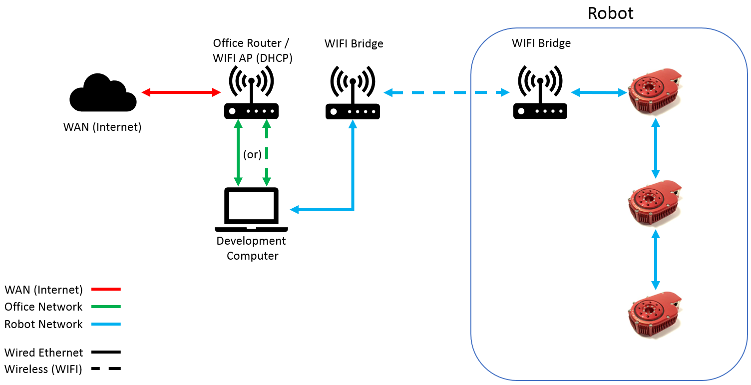
Office Network w/ DHCP + Wireless Bridge |
|
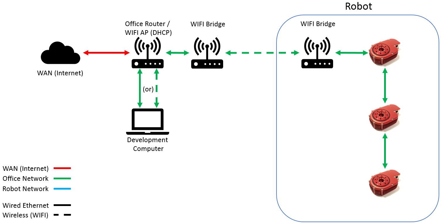
Office Network w/ DHCP + Dedicated Wireless Bridge |
|
Robot Network w/ Static IP |
|
Robot Network w/ Static IP + Dedicated Wireless Bridge |
|
Robot Network w/ DHCP |
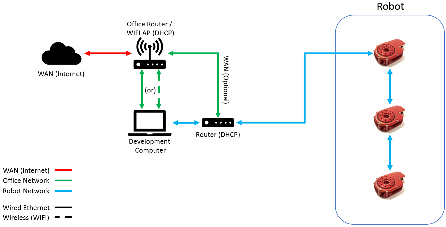
|
Robot Network w/ DHCP + Wireless Bridge |
|
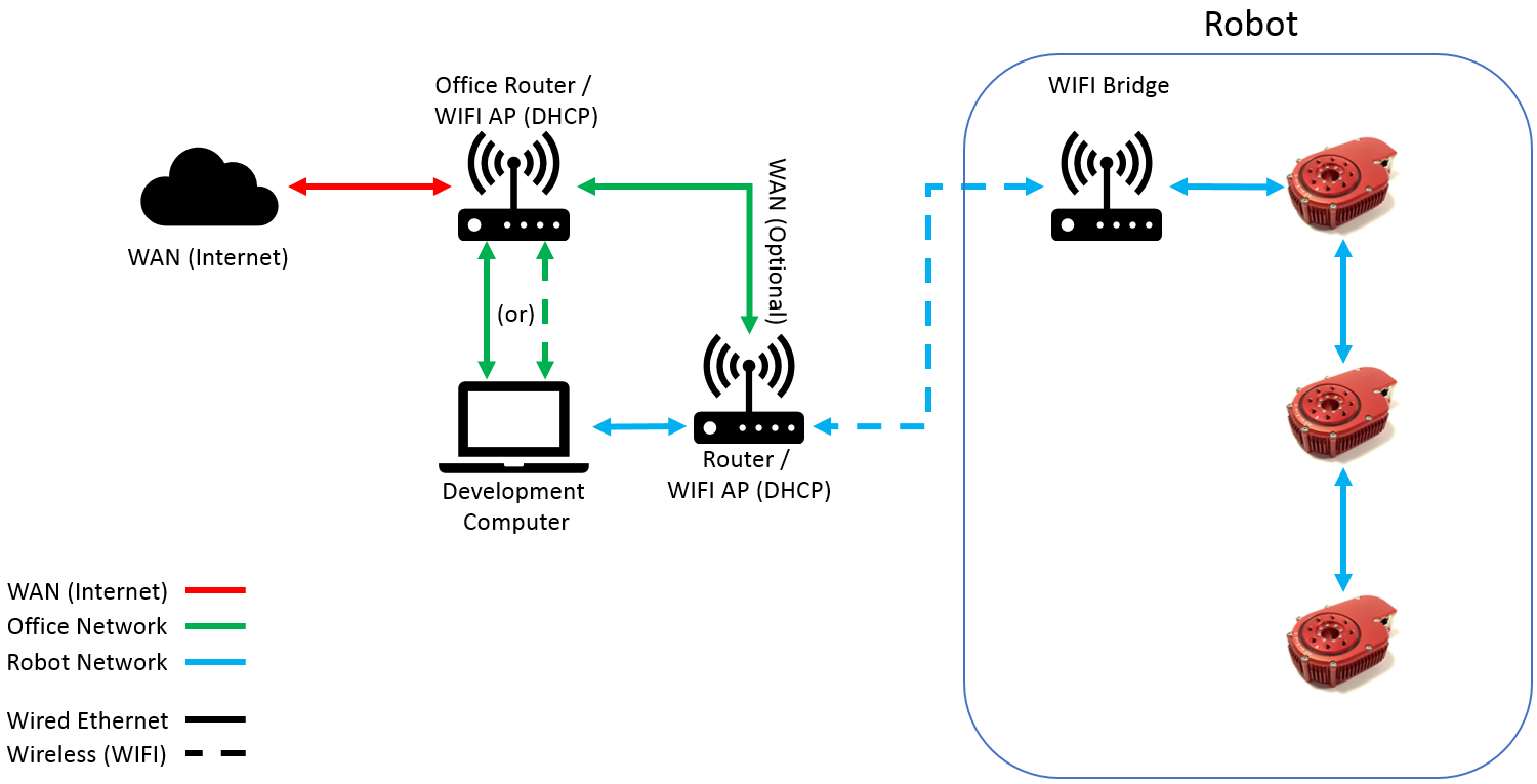
Robot Network w/ DHCP + Dedicated Wireless Bridge |
|
Robot Network w/ DHCP + On-Board Computer |
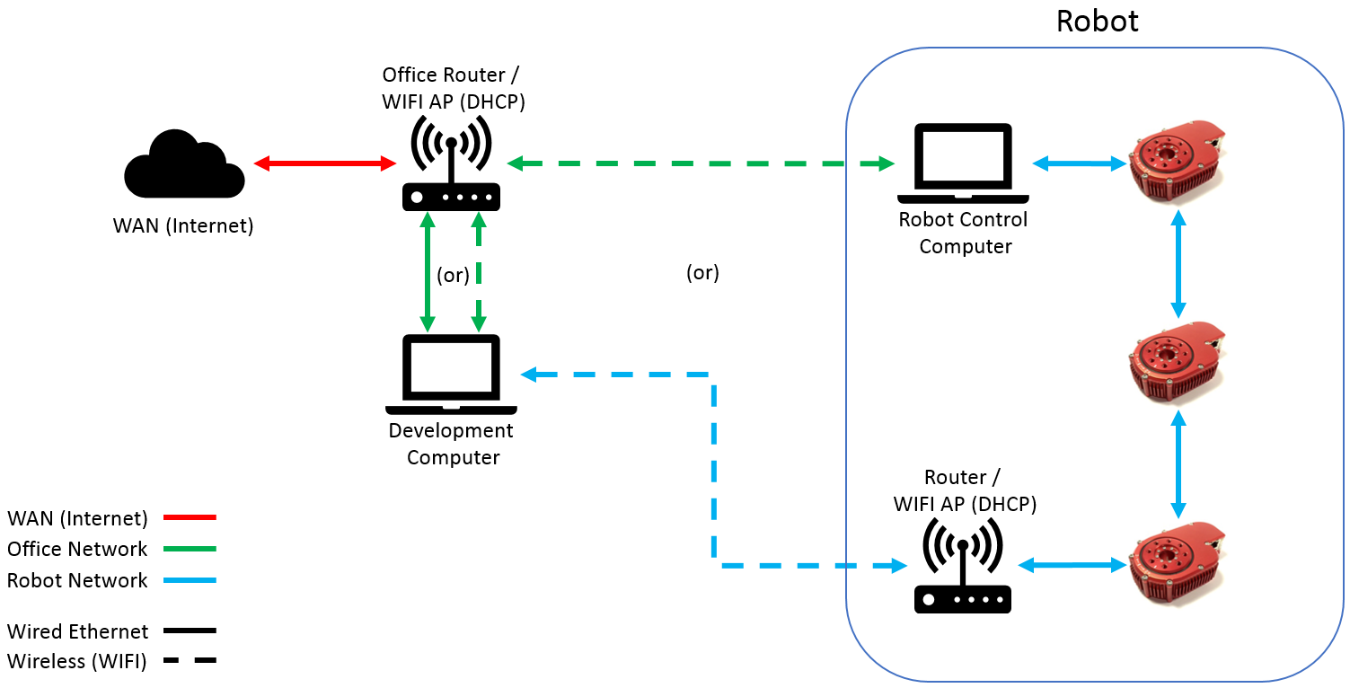
|
Robot Network w/ DHCP + On-Board Computer + Switch |
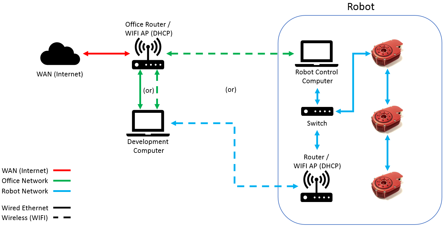
|
Robot Network w/ DHCP + On-Board Computer + Router/Switch |
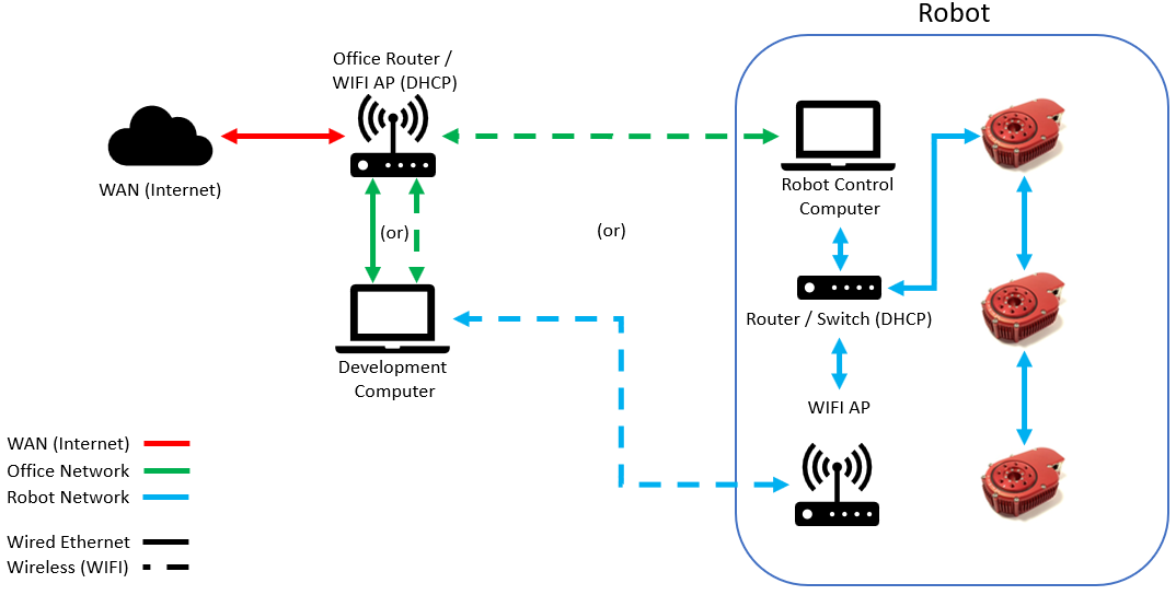
|
Robot Network w/ DHCP + On-Board Computer + Router/Switch/AP |
|
Power
Modules run on DC voltages between 24V-48V. The internal electronics of the modules are designed to properly regulate and automatically scale motor control parameters as the bus voltage changes.
However, if actuators are heavily loaded and are being back-driven or impacting the world with significant amounts of force there may be voltage spikes as energy is sent from a back-driven actuator out into the power system. In these cases we recommend using a shunt regulator, or using a large battery system that can absorb these effects.
LED Status Codes
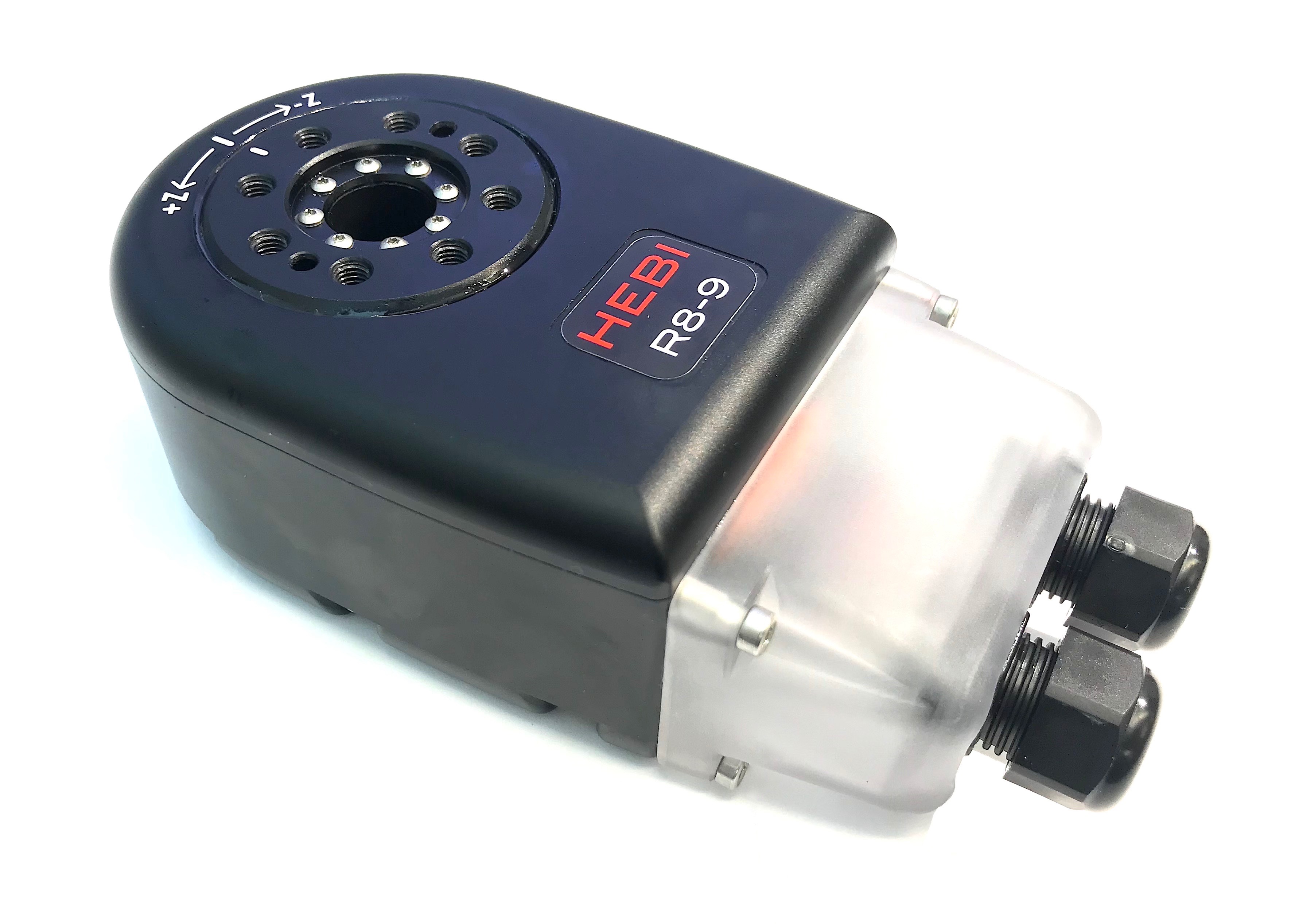
The Status LED is a multi-color indicator that provides information about the current state of a module, detailed in the table below. It is located under the white plastic window on the side of the module near the connector. There is also a smaller white LED to the left of the Status LED that indicates that module is receiving power.
Normal Statuses
The following LED statuses are displayed during normal operation, and common fault or safety modes.
| LED Pattern | Meaning |
|---|---|
Orange/Green Blink |
Not yet obtained an IP address. By default, this is the status of a module when resetting or powering up. After the module receives and IP address, typically after a few seconds, the status LED will change to a Green Slow Fade (see below). Note: For a module to receive an IP address it needs to be on a local network with a router running DHCP. Note: If a module remains in this mode for more than a few minutes without a network connection, and then a network connection is established, the module may not receive an IP address. Restarting the module with an established network connection will solve this issue. |
Green Slow Fade |
Operating normally, not receiving any commands. Note: If a module has a manually assigned IP address it will start directly into this mode when resetting or powering up. |
Green Fast Fade |
Operating normally, acting on received commands. |
Yellow Fast Blink |
M-stop triggered. |
Orange Fast Blink |
One or more of the actuator’s settable position, velocity, or effort limit safety controllers is activated. Position Limits: If an actuator boots up and it is outside a position limit, commands will be disabled until the module moved manually inside the limit. If a new joint limit is set and the module is outside the new limit, commands will be disabled until the module moved manually inside the limit. In the The safety controller documentation has more information about position limits. |
Red Fast Blink |
Motor winding temperature is high, and the motor’s power is being limited by an internal motor thermal safety controller to less than what is currently being commanded from the actuator’s PID controllers. |
Red/Green Fast Blink |
Obtained a bad IP address. This can occur if a module was given a static IP that represents the broadcast (e.g. X.X.X.255 with a subnet mask of 255.255.255.0) or network address (e.g. X.X.X.0 with a subnet mask of 255.255.255.0) on the given subnet, or if it is assigned such an address by the router when set to DHCP mode. |
Bootloader Mode
The following LED statuses are displayed during normal operation when a module is restarted into bootloader mode, which allows the firmware of the module to be updated. Entering this mode, updating, and rebooting is typically handled automatically by Scope.
| LED Pattern | Meaning |
|---|---|
Orange/Light-Blue Blink |
Not yet obtained an IP address. Note: For a module to receive an IP address it needs to be on a local network with a router running DHCP. Note: If a module remains in this mode for more than a few minutes without a network connection, and then a network connection is established, the module may not receive an IP address. Restarting the module with an established network connection will solve this issue. |
Light-Blue Fade |
Abnormal Statuses
The following LED statuses are not encountered during normal operation. If you see any of these on module, please contact us at: support@hebirobotics.com.
| LED Pattern | Meaning |
|---|---|
Green Slow Blink |
Operating normally, but effort (torque) sensing has not been calibrated. Note: This is a hard on-off blink, as opposed to the slow gradual fade that means the module is running normally (see "Green Slow Fade" above in Normal Statuses). |
Yellow Solid On |
Module electronics above safe temperature. |
Red Solid On |
If encountered immediately after exiting the bootloader, the module does not have application firmware. Use the Scope GUI to install new firmware. If encountered while the module is running normally, the motor winding temperature is above a critical value and power to the motor has been shut off. |
Blue Fast Blink |
Current sensing is not calibrated. The module’s motor will drive in this mode. |
Blue Slow Blink |
Position sensing is not calibrated. The module’s motor will only drive in |
No Light |
There is a problem with the module. |
Groups
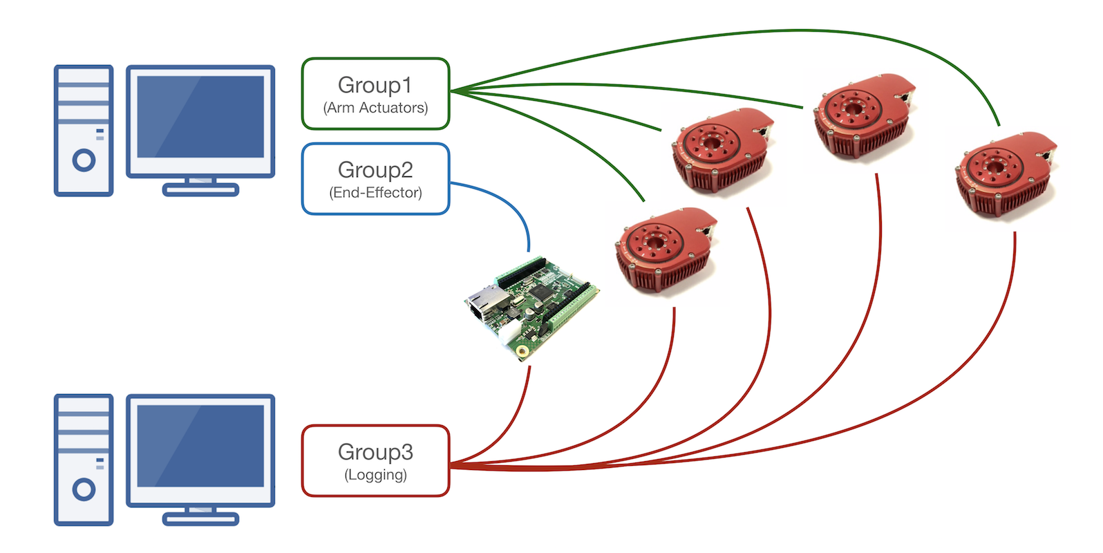
Groups are the way you communicate with modules when using the programming APIs. It allows one or more modules to be treated as one coordinated system in terms of feedback and control. Modules in a group don’t need to be a physically connected "robot". Any modules that are one the same network can be part of a group.
Creating Groups
You create a Group using a Lookup to see what’s on the network. You can adjust settings like the CommandLifetime and FeedbackFrequency.
Once one or more modules are turned on and plugged into the network they can be discovered by a Lookup that periodically sends broadcast messages on the network. The interval is configurable and by default is set to 5 Hz. Each module has a user-settable Name and Family to help better organize a system on the network. These can be set from the APIs or by right-clicking modules in the left panel in the Scope GUI.
Discovered modules can be combined into a Group that provides a basic way to send commands and retrieve feedback. Groups also handle higher-level issues such as data synchronization and logging. You can also request Info from the modules in a group.
Each module has multiple keys that can be used to identify a module on a given network:
-
Family(human settable, e.g., "RobotArm_6DoF") -
Name(human settable, e.g., "base" or "elbow") -
IP address(network unique) -
MAC address(global unique)
There are no software limits on the number of active groups, the number of modules within a group, or the number of groups that a module is part of. Groups are the only way to communicate with modules using the APIs. Even if you are working with a single module, you will need to create a group for that module.
Group Creation Rules
The APIs allow you to create a Group from a Lookup using queries about their Family, Name, and MAC address. For example, you can create a Group of all modules with the Family of HEBI with code such as:
group = HebiLookup.newGroupFromFamily('HEBI')`The most commonly used group create function uses families and names, and can optionally use wildcards for each of these. For example, to get all wrist modules on an arm, one might write:
group = HebiLookup.newGroupFromNames({'HEBI'}, {'Wrist*'})You can even have more complex queries:
% Finds the "Shoulder" and all "Wrist" modules with family "HEBI".
group = HebiLookup.newGroupFromNames({'HEBI'}, {'Shoulder', 'Wrist*'})
% Finds all "Shoulder" and "Wrist" modules from "RobotA", all "Wheel"
% modules from "RobotB", and all other modules which have a family name
% starting with "HEBI".
group = HebiLookup.newGroupFromNames({'RobotA', 'RobotA', 'RobotB', 'HEBI*' }, {'Shoulder*', 'Wrist*', 'Wheel*', '*'})
This can look confusing, but the behavior is well defined for vectors of family and name inputs. The rules followed by the APIs are listed below; F is the number of elements in the family vector and N is the number of elements in the name vector:
-
If either one of the vectors is length one, then the one element in that vector gets repeated so the vectors are the same length.
-
If
F != N, an error is thrown. -
The entries are treated as
(family | name)pairs. Each pair tries to match all modules that have been found on the network. -
if
nameorfamilydoes not contain a wildcard, the matcher must return exactly one result; otherwise, it can return more than one. Otherwise, an error is thrown. -
matches generated by wildcards are sorted alphabetically, first by family, then name, then MAC addres.
-
once all pairs have been processed, the entire list of matched modules is checked for duplicates (a module matched by two or more family/name pairs). If any are found, an error is thrown.
If no error is thrown, a group is returned with all of the matched modules.
Feedback
You get synchronized Feedback from a Group. Once a Group is created, feedback requests automatically go out to all the individual modules and actuators in the group at the FeedbackFrequency and get organized by the API into vectors, matrices, and structures of data corresponding to all the feedback from a single point in time.
You can view the most recent feedback for a group at any time by getting the NextFeedback for the group. The details of how NextFeedback is returned are API-dependent.
Feedback contains things like the position/velocity/effort of an actuator, the states of various input/output pins of an I/O board, and a wealth of other sensors and internal module state. The complete details of what is returned in module feedback is specific to the particular hardware or software application and are documented in the sections below:
Commands
You can send Commands to a group, typically desired position, velocity, and effort commands, for actuators to execute. These commands are targets for low-level controllers that run on an actuator. Commands are typically sent from a loop that runs around 100 Hz, but you can run faster (up to 1kHz) or slower depending on the needs of your application. Generating smooth commands to go from one position to another can be accomplished the Trajectory API.
Actuator Commands
| Parameter | Units | Description |
|---|---|---|
|
|
The desired position of the output of an actuator. |
|
|
The desired velocity of the output of an actuator. |
|
|
The desired torque or force of the output of an actuator. For an actuator in |
Clearing Commands
To stop commanding an actuator, or to send commands to only certain actuators in a group, the APIs make use of NaN to indicate no active actuator command. For example to only command positions of 90 degrees to the first and last actuators in a 4-actuator group while sending no commands to the middle actuators, the command would be:
position_cmd = [ pi/2, NaN, NaN, pi/2 ]
For effort commands it should be made clear that commanding NaN is distinctly different from commanding 0. An effort command of NaN will clear any commanded effort, and if that is the only command to the actuator there will be no motor output, as all the PID controllers will be inactive. A command of 0 effort will cause an actuator to actively servo its output to maintain zero-torque.
|
Command Lifetime
For safety, each command has a CommandLifetime. This is the maximum duration that a command may be active before it expires. If the hardware does not receive further commands within the specified time frame, all local controllers get deactivated. This is similar to a safety feature that many industrial robots have that requires users to send at least one update every interval (e.g. 5 ms) to keep the robot from turning off and locking up. Since the timeout deadline depends heavily on the application, we chose to implement the inverse approach in which every command specifies its own lifetime.
Additionally, modules do not accept commands from any other sources during the lifetime of a command. This lock-out mitigates the risk of other users accidentally sending conflicting targets (e.g., by dragging slider in the Scope GUI). The default command lifetime in all APIs is 0.25 sec. You can set CommandLifetime to be any value greater than 0. Setting CommandLifetime to 0 is a special case that disables it. This means that commands sent once will be active on a module indefinitely, and that a module will also accept commands from other sources, since there is no lock-out.
While the timeout can be deactivated, we strongly recommend to make use of this feature. Otherwise, the hardware will continue to execute the last sent command indefinitely, which can result in unwanted behavior, especially when commanding velocities and efforts (torques). Alternatively, we recommend using a hardware button that triggers a motion stop ("M-Stop").
Note that the command lifetime is a common source of confusion for new users. If commands are only sent once, or if your program pauses for longer than CommandLifetime between sending commands, a module will stop until a new command is sent. In normal use of the API commands should be sent in a loop, typically around 100 Hz.
|
Logging
You can log feedback automatically in the background at the group’s FeedbackFrequency. These logs can be loaded into memory or converted into different formats for use with other tools. Each Group can be generating one log at a time. It is possible (and often useful) to have more than one group simultaneously gathering feedback and/or logging from the same modules.
Logs are stored in a binary format and by default are labeled with a .hebilog file extension. Logging begins with a startLog call that returns the path to the .hebilog file and ends with a stopLog call. Calling startLog on a group that is already logging will immediately stop the current log and start a new one. Each API has tools that can load and parse logs into organized formats.
Settings and Info
You can also use the APIs to set a number of different module-specific parameters, such as Gains and Safety Limits. See the Hardware Documentation for more detail.
Motion Control
![]()
![]()
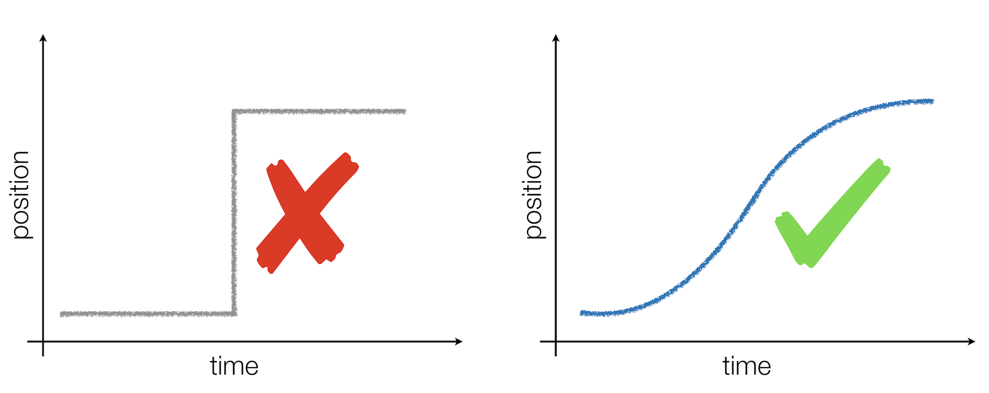
HEBI actuator modules can be controlled using position, velocity, and effort (typically torque). This section discusses the details of how these different inputs can be controlled and tuned for specific applications. Typically, the best performance can be achieved by coordinating and controlling a combination of commanded positions, velocities, and effort. The plots above show the difference between a poorly tuned controller (left) and a well-tuned controller (right) tracking the same desired commands.
Control Strategies
Position, velocity, and effort controllers can be run individually or in any combination simultaneously. To combine these control inputs, PID control loops are used on position, velocity, and effort. These controllers can be cascaded and combined in different preset configurations, termed Control Strategies.
| We generally recommend using Strategy 4. More details are provided in the section on gain tuning. |
The active Control Strategy and its corresponding parameters can be set using:
-
Any of the APIs.
Changes to the active control strategy on an actuator do not automatically get persisted and will revert back to their original values after a rebooting a module. Settings on a module can be persisted by right-clicking the actuator in the Scope GUI or via the persist command in the various APIs.
|
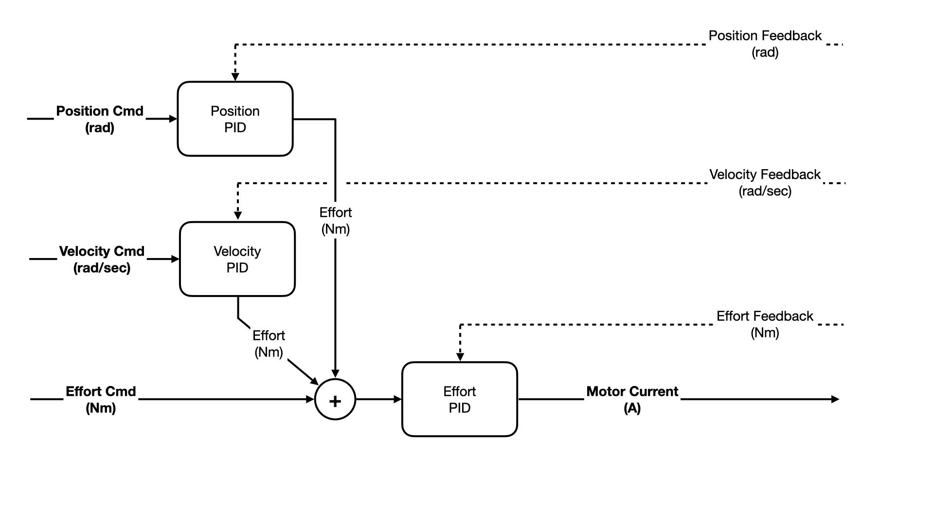
Strategy 5
H-Series Actuators and Motor Drivers
This controller is used for actuators that support field oriented control (FOC) of motor current. Position and Velocity PID outputs sum with a feed-forward effort signal to generate an intermediate effort signal. This intermediate effort signal is then passed through an "inner" Effort PID controller which generates a commanded motor current.
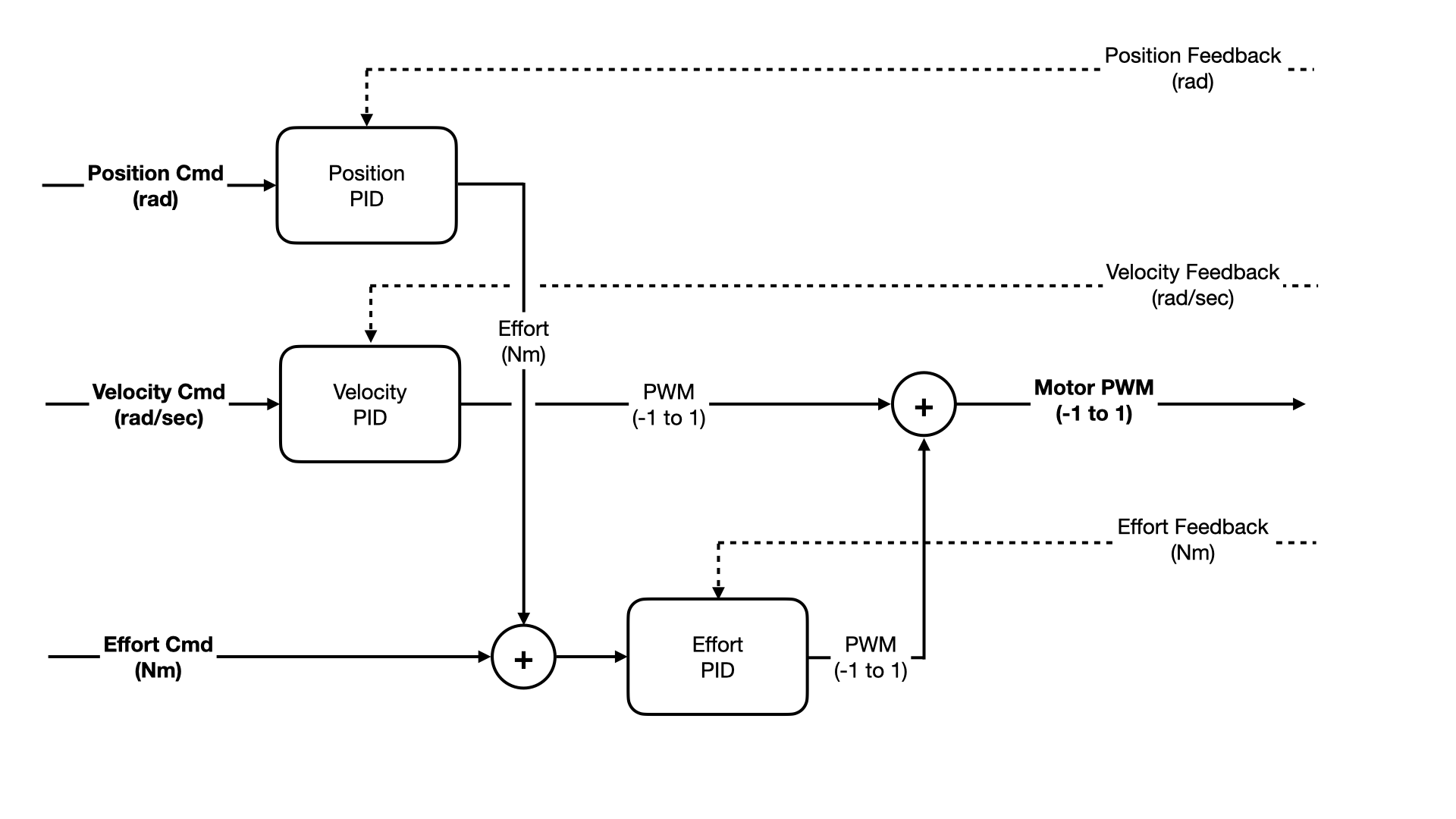
Strategy 4
X/R/T-Series Actuators and Motor Drivers
This controller is used for actuators that support motor PWM control and block commutation. Position PID output sums with a feed-forward Effort signal to generate an intermediate Effort signal. This intermediate Effort signal is then passed through an "inner" Effort PID controller. The PWM output of the inner Effort controller is added to a Velocity PID controller output to generate a commanded motor PWM (voltage).
Strategy 3
Legacy - Not Recommended
Position, Velocity, and Effort PID controllers all directly sum to generate motor PWM commands.

Strategy 2
Legacy - Not Recommended
Position and Velocity PID outputs sum with a feed-forward effort signal to generate an intermediate effort signal. This intermediate effort signal is then passed through an "inner" Effort PID controller which generates motor PWM commands.

Direct PWM
X/R/T-Series Actuators and Motor Drivers using Block Commutation
A PWM command is set directly, from -1 to 1. This controller uses no feedback from the sensors in the actuator. The controller does not compensate for changes in the supplied voltage.
All safety controllers to protect the actuator (temperature, velocity, joint limits, etc.) are still applied.
Direct FOC
H-Series Actuators and Motor Drivers using FOC
A commanded motor current in Amps is set directly for both I_q (torque generating current) and I_d (non-torque generating current). This controller uses no position/velocity/effort feedback from the sensors in the actuator. However, it does use the motor phase current sensors to provide closed-loop current control as configured with the FOC Torque Control gains in the Motor Driver Tab in Scope.
Commanded motor V_q and V_d voltages can also be directly applied.THis is typically without commanding I_q and I_d currents, as the FOC controller will typically wind up overriding these commands.
All safety controllers to protect the actuator (temperature, velocity, joint limits, etc.) are still applied.
Off
The motor is turned off. The actuator will not respond to commands of any kind.
If the actuator is equipped with a mechanical brake (some H-Series models) it will engage, locking the actuator.
Safety Controllers
In all of the control strategies, a series of safety controllers run after the calculation of the final PWM values (the 'Motor PWM' value in the control strategy diagrams above). These safety controllers will potentially modify the PWM value based on things like the bus voltage, motor winding temperature, motor velocity, and position limits.
The diagram below shows the priority in which the safety controllers run. Safety controllers that are applied later in the chain (further to the right in the diagram) take priority over safety controllers that are applied earlier (further to the left). Some of these safety controllers are parameterized and can be set by the user, such as the position safety limits. Other controllers, such as the voltage limit and motor temperature limits, are fixed and are set specifically for a certain type of hardware.

The configurable safety controllers (such as the position limit strategy and its corresponding limit values) can be configured from:
-
The Gains Tab in Scope
-
The Motor Driver Tab in Scope
-
Any of the APIs
Position Limits
Position limits can be set in firmware independently for the lower and upper bound of the allowed motion. To remove a limit, use +/- infinity (for the upper and lower limit respectively); in Scope this is represented by inf or -inf. Invalid configurations (e.g., a upper bound of -1 and lower bound of +1) are ignored by the modules.
When the module exceeds its position limit, the LED flashes orange.
There different strategies that can be activated when an actuator is at its position limit, detailed in the table below.
| Strategy | Description |
|---|---|
Disabled |
In this strategy, position limit values can be set and stored, but do not affect control. |
Damped Spring |
This strategy acts as a virtual spring, actively pushing the module back inside when it exceeds the set limit value. If the module boots up outside of the configured position limits, it will not exert any output force until it is manually moved back inside the range (or the limits are configured so that the current position is inside the range). When outside the position range, commands are ignored unless their net effect is to direct the module back inside the range of valid positions. For firmware earlier than v15.0.0, this is the default and only supported mode. |
Hold Position |
When the module is set to Hold Position, then the module attempts to control the output to hold the current position if the configured limit is exceeded (similar to the hold position M-stop strategy). To recover from this limit behavior, the position limit must be set to Disabled, the module moved inside the configured position limit range, and then reset to Hold Position. |
Motor Off |
When the configured limit is exceeded when in Motor Off, the control strategy is changed to Off, so the module does not actively control the output and commands are ignored. As with the Hold Position strategy, a semi-manual reset is required. The module should be moved back into the valid position limit range, and then the control strategy restored from Off to whatever the previous control strategy was. |
M-Stop Strategies
In addition to safety limits, actuators also support a Motion-Stop that can be triggered by pressing an external hardware button. The trigger action can be chosen by setting one of the following m-stop strategies.
| Enabling the motion stop does require additional hardware components. |
| Strategy | Description |
|---|---|
Disabled |
In this strategy, triggering the m-stop has no effect. |
Motor Off |
When the m-stop is triggered when in Motor Off, the control strategy is changed to Off, so the module does not actively control the output and commands are ignored. In order to resume control, the m-stop has to be un-triggered and the control strategy has to be manually restored by the user. |
Hold Position |
When the module is set to Hold Position, then the module attempts to control the motor to hold the current motor position if the m-stop is triggered (similar to the hold position limit strategy). The control strategy does not change, and normal operation continues as soon as the m-stop is un-triggered. |
Parameters and Gains
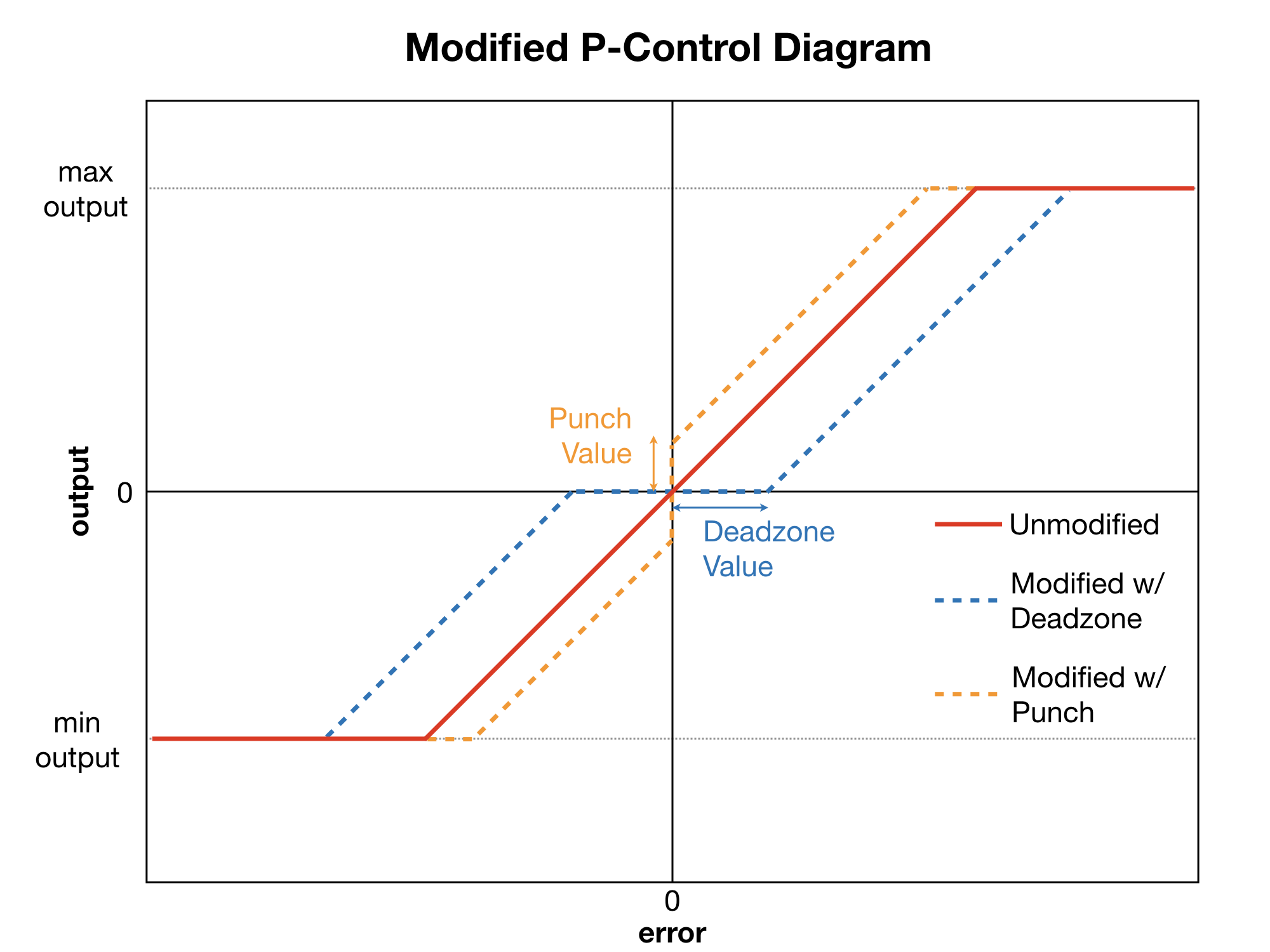
Each controller for position, velocity, and effort is a full PID controller that exposes gains for tuning the proportional, integral, and derivative response of the control loop. Additionally, there are are number of other parameters that can be used to modify the response of the loop (see table below), threshold and low-pass the input and output, limit integral windup, set a deadzone region, and provide feedforward commands where appropriate.
A diagram showing the effect of min/max output limits, deadzone, and punch parameters on a standard proportional controller (P-controller) is shown below.
Description of Parameters
The table below lists the parameters that are common to each of the individual position, velocity, and effort PID-controllers. The API-specific information for each parameter are detailed in the next section.
The gains and control parameters on a module can be set using:
-
Any of the APIs.
|
Changes to the gains on an actuator do not automatically get persisted and will revert back to previously persisted values after a reboot. Gains and other module parameters can be persisted by right-clicking the actuator in the Scope GUI or via the |
| Parameter | Description | Units |
|---|---|---|
|
The proportional gain of a standard PID-controller. The role of this term is to act like a linear spring and provide an output proportional to the measured error. |
|
|
The integral gain of a standard PID-controller. The role of this term is to accumulate past errors to help eliminate steady-state error. |
|
|
The derivative gain of a standard PID-controller. The role of this term is to damp the error based on its velocity. |
|
|
Feedfoward gain that is multiplied to the input value. If the PID controller is a velocity or effort controller that outputs |
( |
|
Area around zero where the output of the PID loop is modified to reduce its output. The deadzone will shift the effect of |
|
|
Maximum value that |
|
|
A step amount that can be added to the standard proportional gain that can sometimes be useful in overcoming motor stiction. |
|
|
Threshold values for the input to the PID controller. |
|
|
Threshold values for the output to the PID controller. |
|
|
A IIR low-pass filter applied to either the input to the PID controller. |
|
|
A IIR low-pass filter applied to either the output of the PID controller. |
|
|
Flag for whether |
|
Choosing a Control Strategy
| Control Strategy | Notes |
|---|---|
Strategy 5 |
This is the recommended control strategy for H-Series Actuators and Motor Drivers that are configured for FOC. The position and velocity controllers command a desired torque and the output of the effort controller is a desired winding current at the motor. |
Strategy 4 |
This is the recommended control strategy for X/R/T-Series Actuators and Motor Drivers that are configured for Block Commutation using hall sensors. The position controller commands an inner effort (torque) controller. This has the advantage that the gains on the position controller are more intuitive units of [Nm / rad error]. Additionally, the inner effort controller allows the actuator to be more actively compliant and respond much more like a linear spring in its position error. If you are concerned primarily with position/velocity tracking, and less about compliance and force control, you may want to remove the effect of feedback from the actuator’s torque sensing. Do do this, you can set the Kp / Ki / Kd terms on the effort controller to 0, being sure to leave the Feed Forward term at 1. This will give you the same properties as what was provided in Strategy 3, but with more intuitive gains on position control. This will also let you cap the commanded torque to the inner loop by setting the Output Min / Max of the position controller. In this strategy the velocity contoller also feeds directly to motor PWM. Because of this, the velocity PID loop can apply a feedforward PWM to the motor based on the desired velocity and the known actuator parameters. This allows Strategy 4 to have better velocity control with lower |
Strategy 3 |
No longer recommended. As its advantages for position/velocity control can be more easiliy achieved by adjusting the effort control loop gains in Strategy 4. |
Strategy 2 |
Good for control if you want the velocity controller to act as much as possible as a linear damper (viscous damping). We have generally not favored this control strategy for most applications because the noise in the velocity feedback signal makes for poor control when resulting effort command from the velocity PID controller is fed to the effort controller. |
Direct PWM / |
Use if you want to run your own position / velocity / effort control at the API level in a way that isn’t satisfied by the built-in controllers on the actuator or module. It is also useful for system identification of the actuator or debugging purposes, since it elimates all feedback control within a module. |
Tuning Controller Gains
Performance of an actuator or an overall robot depends heavily on the settings of the controller parameters, or 'tuning the gains'. HEBI actuators ship with a set of default gains that allows the actuator to run well under light loads, but if a significant load or inertia is added to the actuator’s output the gains that are needed for good control will likely change.
For some single-DOF systems there are a variety of standard gain-tuning techniques can possibly be applied. Finding 'good gains' for something as complex as a full robot depends on the details of the desired application. For new multi-DOF systems it is difficult to predict ahead of time how the gains will need to be tuned. However, there are some rules of thumb:
-
Lower is better. If a system can perform well with lower gains, that is often preferable for safety, stability, and efficiency.
-
Rather than command only positions, calculate desired velocities and command those as well. Especially in Strategy 3 and 4, this can dramatically improve tracking of commands without relying as much on a high Kp on position.
-
The gains of the effort (i.e. torque) controller generally do not have to be tuned much from their default values. The gains on the position and velocity controllers are usually where most of the tuning occurs.
-
When commanding velocities, set the the Kd on position to 0, since the Kp on velocity will serve the same purpose.
-
In some cases, low-passing the outputs of the PID controllers (particularly the torque and velocity controllers) can provide more stable control, at the expense of lag in the output.
-
In the case of a robot arm, the proximal actuators closer the base that bear more load will generally have higher position and velocity gains than the more distal actuators out at the wrist.
-
Use commanded effort, rather than high integral gain on the position controller, to handle disturbances that can be modeled for your robot. This is often things like gravity compensation for an arm.
-
Make use of the PWM plot in the Scope GUI, or the commanded PWM feedback in the APIs, to understand how the controllers are responding and combining during tuning. For example this plot can indicate if there is jitter from aggresive gains on a noisy proportional or derivative signal, or how quickly an intergral term is winding up.
Kinematics
In each API, we provide libraries and tools that help calculate and solve problems related to a robot’s kinematics. These tasks include things like calculating forwards kinematics and Jacobians, as well as solving inverse kinematics. In addition to kinematic information that describes the physical geometry of a system, our APIs provide basic information (mass and inertias of each body) about the robot’s dynamics. This aids in calculating the torques and forces needed for tasks like gravity compensation, balancing, or quick movements.
Body Types
The kinematic structure of the robot can be specified using built-in body types. A body can be either a static component (e.g. link) or a dynamic component (e.g. joint). Currently, our kinematics APIs only support serial chains of these bodies.
Parameterized body types are built-in to each API and correspond to components on our parts list. Please refer to the language-specific API documentation for more information on using these libraries in your application. While the types and parameters for setting up kinematics are consistent across APIs, the concrete implementation does depend on the language.
Kinematics Setup
The first step in using the kinematics API is to configure the robot by adding bodies together in a kinematic chain. The details are API-dependent, but the overall idea is to form of chain of actuated joints, connected by passive links. The APIs have functions for quickly defining and parameterizing HEBI actuators and accessories as well as functions to fully define custom links and joints.
Additionally, you can save and load kinematic descriptions to and from files using the HEBI Robot Description Format.
The last body of the chain is considered to the the end-effector. All the coordinate frames for kinematics are expressed in the BaseFrame. The first body in the kinematic chain is by default at the origin of the BaseFrame. If desired, it can be set to be something different.
Forward Kinematics
Forward kinematics refers to calculating the pose (position and orientation) of various bodies on the robot based on a given configuration (a set of joint positions).
Once the bodies of a robot are configured, the API can return the forward kinematics of the robot for a given set of joint positions as [4 x 4] homogeneous transforms in the base frame. In the case where the frames of multiple bodies are returned (e.g. the output frames of each body in the robot for visualization) they are returned as m [4 x 4] 3D matrix where m is the number of bodies in the robot.
Jacobians
In robotics, the Jacobian, \(\mathbf{J}\), refers to a matrix that relates the velocities, \(\dot{\theta}\), of a robot’s joints, \(\theta\), to the velocities, \(\mathbf{v}\), (both linear and rotational) of various bodies of the robot, the typical case being the body that is the end effector of an arm. It also relates the torque of a robot’s joints, \(\tau\), to the forces and torques, \(\mathbf{f}\), on different bodies.
The Jacobian has the following relationships:
| Equation | Explanation | Typical Use Case |
|---|---|---|
\(\mathbf{v} = \mathbf{J} \dot{\mathbf{\theta}}\) |
Body velocities equals the Jacobian times the joint velocities. |
Given a robot’s joint velocities, find the resulting end-effector velocities. |
\(\mathbf{\dot{\theta}} = \mathbf{J}^{-1} \mathbf{v}\) |
Joint velocities equals the inverse of the Jacobian times the body velocities. |
Given desired end-effector velocities, find the appropriate robot joint velocities. |
\(\mathbf{\tau} = \mathbf{J}^{T} \mathbf{f}\) |
Joint forces/torques equals the Jacobian-transpose times the body forces/torques. |
Given a desired force/torque at the end-effector, find the appropriate robot joint torques. |
\(\mathbf{f} = (\mathbf{J}^{T})^{-1} \mathbf{\tau}\) |
Body forces/torques equals the inverse of the Jacobian-transpose times the joint forces/torques. |
Given a robot’s joint torques, find the resulting end-effector forces/torques. |
The Jacobian itself is a matrix of partial derivatives, defined at a given set of joint angles. The size of the Jacobian is [6 x n] where n the number of joints (degrees of freedom, of DoF) in the robot. Rows 1-2-3 of the Jacobian relate respectively to the X-Y-Z translation of a body, and rows 4-5-6 relate respectively to the X-Y-Z rotations of a body, all expressed in the base frame.
So in the equations above the vector of forces, \(\mathbf{f}\), and the vector of velocities, \(\mathbf{v}\), are:
Once the bodies of a robot are configured, the API can calculate the Jacobian to all the different bodies for a given set of joint positions. In the case where Jacobians to multiple bodies are returned (e.g. the Jacobians to the center-of-mass of each body in the robot for compensating for the robot’s dynamics) they are returned as m [6 x n] matrices, where m is the number of bodies in the robot.
Inverse Kinematics
Inverse kinematics (IK) refers to solving for the [1 x n] vector of joint positions that put the end-effector of the robot in a certain pose (position and/or orientation), where n is the number of joints (or DoF) in the robot. This is in general a harder problem than forward kinematics, as there can frequently be multiple IK solutions for a desired pose. Our approach in the HEBI APIs is to use local optimization to find an approximate solution for joint positions, given an initial 'guess' of joint positions.
The APIs allow you to provide different 'targets' for the end effector for IK solver to try to reach. You can combine multiple targets, e.g. you can solve for both the position and orientation of the end effector by specifying both XYZ and SO3. All poses are expressed in the base frame. You can also specify the InitialPositions for where the optimizer to starts.
|
Specifying good If you are running a robot online and calculating IK at regular intverals it is often a good idea to 'warm start' the IK solver with either the commanded or feedback joint positions from the last iteration. The HEBI Arm API> does this by default. If you know roughly the configuation or area of the workspace the robot will be working in, seeding with joint positions in that area will also work. |
| Parameter | End Effector Target | Comments |
|---|---|---|
|
xyz position (m) |
|
|
z-axis orientation of end effector |
|
|
3-DoF orientation of end effector |
|
|
Initial seed for the numerical optimization. This is an important parameter for IK to work well. See above. Defaults to all zeros. |
Trajectories
When controlling motion, it is important to command smooth and feasible motions to move from one pose to another.
For example, suppose you have a robot arm that has picked up an object and needs to move it from one side of a table to the other. This motion needs to take a few seconds to execute. Rather than immediately command the target joint angles that move the arm’s end-effector to the new position, a better approach is to find lots of intermediate joint angles that smoothly move to the target position, gradually speeding up and slowing down. This is what the trajectory API helps you do.
Trajectory Generator
HEBI provides a trajectory generator API that creates smooth trajectories between various sets of joint positions (waypoints). These trajectories have the property that they smoothly accelerate and decelerate with "minimum jerk" and are similar to human movement. The generated trajectories are essentially a set of polynomials parameterized by time that can be evaluated to get intermediate positions, velocities, and accelerations that smoothly move between waypoints. The implementation of our trajectory generator is based on methods that have been developed to control small quadrotors.
In addition to position waypoints, there are additional constraints that can be applied so that the trajectory matches velocity and acceleration constraints at the end waypoints or any intermediate waypoints. For example, if you are controlling the swinging of a leg on a robot you can use the trajectory generator to find a smooth sweeping motion that lifts the leg up and puts it down as well as match a desired foot velocities and lift-up and touch-down.
| While the trajectory API is typically used to generate commands for HEBI Actuators, it is a general-purpose solver that can be used independently of HEBI hardware and other APIs. The trajectory generator can be used to generate workspace paths for the end-effector of an arm, or smooth motions for a mobile base. |
In the table below p is the number of waypoints in the trajectory and n is number of joints (DoF) in the robot.
| Parameter | Definition | Comments |
|---|---|---|
|
|
Normal use is to fully specify all positions. You can manually leave positions 'free' to be solved by the generator by using |
|
|
Values for waypoint timing must be fully specified and monotonically increasing. Time cannot go backwards or have the same value for multiple waypoints. |
|
|
Optional. If not specified, beginning and end waypoints are are assumed to be |
|
|
Optional. If not specified, beginning and end waypoints are are assumed to be |
For motion to come to a full stop at an interior waypoint (any waypoint other than the first or last waypoint), the velocities and accelerations constraints both need to be set to 0.
|
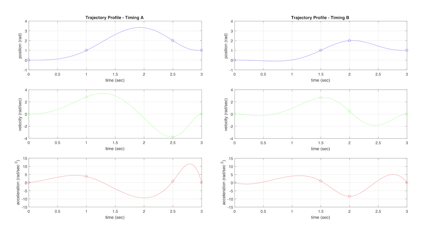
Example: Different Waypoint Timing
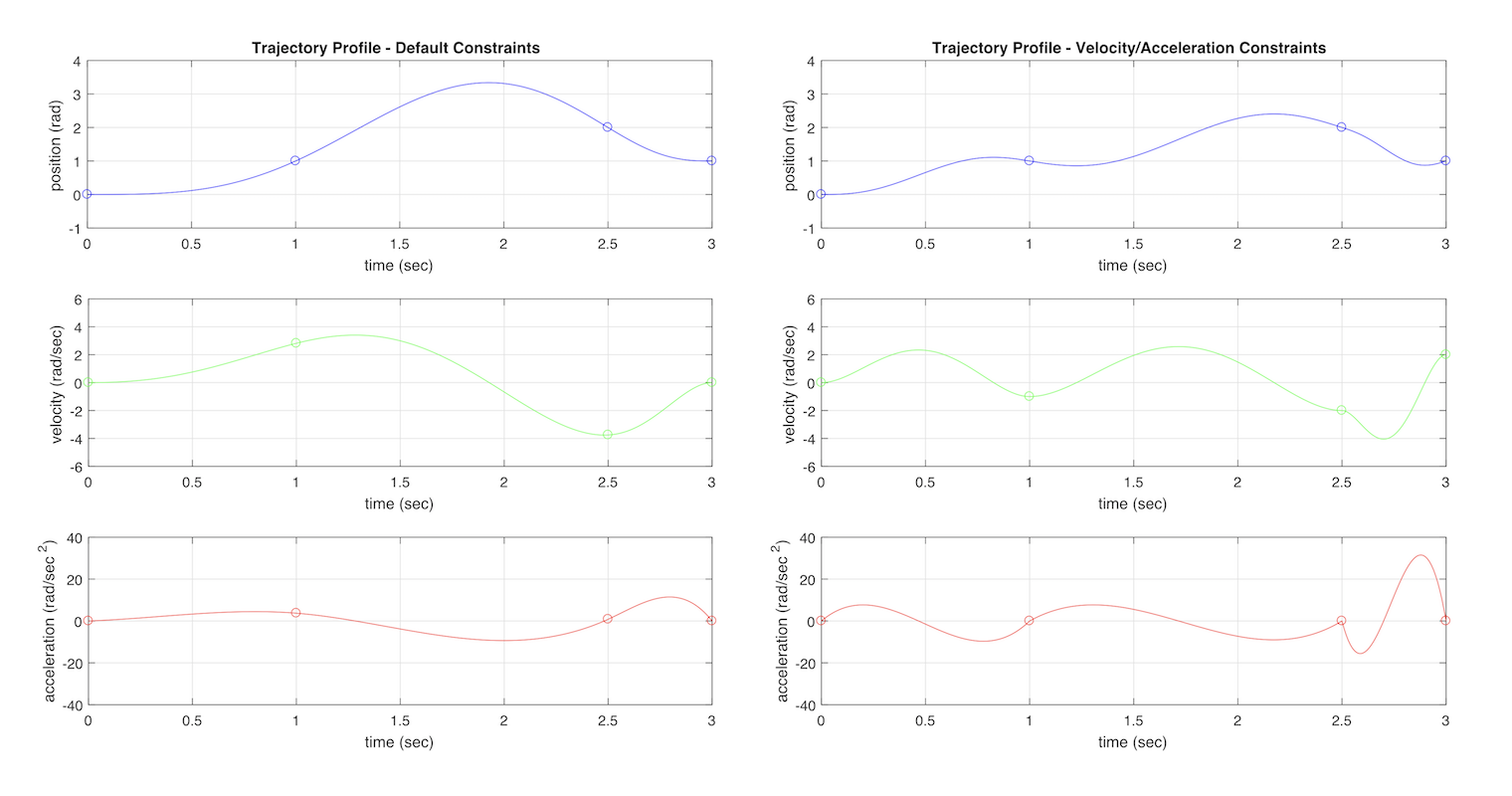
The following plots show examples for two trajectories that have the same waypoint positions but different times. Both trajectories have the default constraints for for velocities and accelerations, which are zero for the first and last waypoints and are left unconstrained for the intermediate waypoints. Note that timing of when to pass through a waypoint can have a significant effect on the shape of the overall trajectory.
| Parameter | Values - "Timing A" (Left Plot) | Values - "Timing B" (Right Plot) |
|---|---|---|
|
|
|
|
|
|
Example: Different Waypoint Constraints
The following plots show examples for two trajectories that have the same waypoint positions waypoint and times. They differ in that the trajectory on the left has additional constraints for velocities and accelerations. Note that manually specifying additional position and velocity constraints can have a significant effect on the generated position trajectory, as well as the peak velocities and accelerations in the trajectory.
| Parameter | Values - "Default" (Left Plot) | Values - "Constrained" (Right Plot) |
|---|---|---|
|
|
|
|
|
|
|
|
|
|
|
|
Executing a Trajectory
After a trajectory has been generated, it can be evaluated at any point in time betwen its first and last values in the times vector. Evaluating a trajectory at a given time will return a set of positions, velocities, and accelerations that smoothly move between waypoints.
-
The
positionsandvelocitiesare typically sent directly to the actuators in a robot using the Group API. -
The
accelerationsare typically passed to other tools or APIs and that use the mass, inertia, and kinematic information for a robot to calculate desiredefforts(torques/forces) that can also be commanded.
Motor Control Modes
There are a few different commutation modes available for use with the HEBI Motor Driver.
Block Commutation
Requirements:
-
Motor Hall Sensors
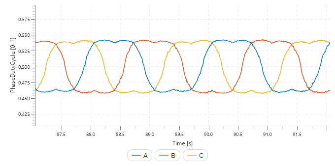
Block Commutation Typical Duty Cycles
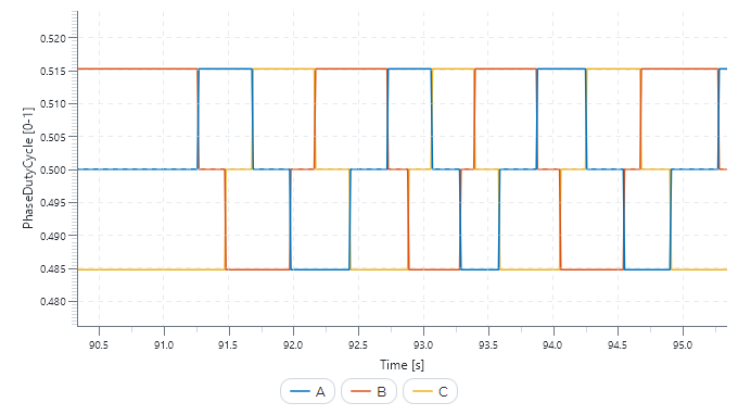
Block Commutation, also known as Six-Step Commutation, drives the motor at a constant voltage.
It utilizes a motor’s embedded Hall Effect Sensors to detect the rotor’s electrical position.
The hall state is derived from the hall sensor inputs as well as the Hall Order and Hall Offset Scope parameters.
hall_state = [A << 2 | B << 1 | C << 0]
table_index = index[hall_state] + hall_offset
As the motor spins, the hall state will update to reflect the new rotor position. At slow speeds you can watch the hall state tick up (or down, depending on the motor direction) from 0 to 5.
Block Commutation Typical Hall States
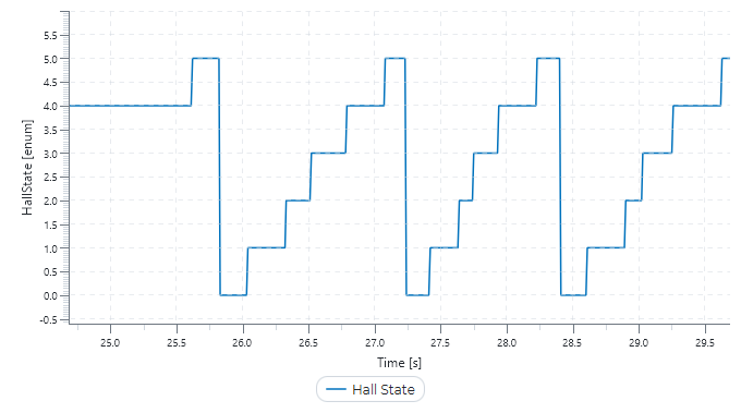
The hall state tells us the Motor Driver what index to use in the excitation table (shifted by 3 depending on the direction).
Excitation Table
| Index | Hall State | Open Phase | Positive Phase | Negative Phase |
|---|---|---|---|---|
0 |
|
C |
+A |
-B |
1 |
|
A |
+C |
-B |
2 |
|
B |
+C |
-A |
3 |
|
C |
+B |
-A |
4 |
|
A |
+B |
-C |
5 |
|
B |
+A |
-C |
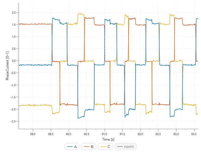
This commutation strategy results in "blocky" winding currents and noticeable torque ripple.
Block Commutation Typical Current Feedback
Field Oriented Control
Implementation Requirements:
-
High Resolution Motor Encoder
-
Motor Encoder Offset Calibration
-
FOC PI Loop Gains
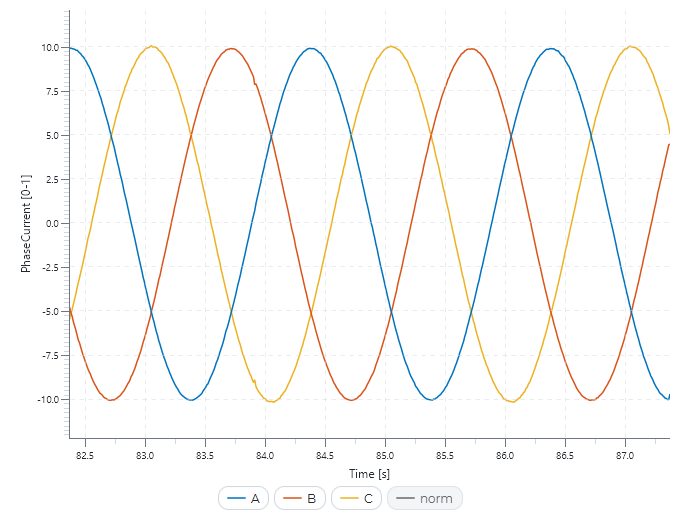
FOC Typical Duty Cycles
Field Oriented Control, often abbreviated to FOC, drives the motor at a constant current. It uses a high-resolution measurement of the rotor position to generate sinusoidal currents in the motor. This results in higher efficiency, torque output, and lower electrical noise.
FOC Typical Currents
All of these advantages don’t come for free - FOC is much more complicated and computationally demanding compared to Block Commutation. FOC requires good current estimates, an encoder calibration, and tuned PI gains.
FOC Appendix
Technical Implementation Details
The HEBI Motor Driver firmware utilizes the Power-Variant (Scale-Invariant) version of the DQZ transform to run the FOC loop. It then uses Space-Vector-Modulation with Midpoint-Clamped Overmodulation to convert phase voltage commands into duty cycles. The FOC loop runs at an integer divisor of the switching frequency in a high speed interrupt immediately after the winding currents are sampled.
The winding currents are measured using a dedicated low-side current sense amplifier on each phase. Winding currents are sampled in the middle of the on time of the low side FETs.
The phase voltages are measured directly at the output of the PWM stage through a low pass filter. This works well for sensing back EMF when the power stage is off but does not work very well when the switching stage is on.
Contact support@hebirobotics.com for more details.
FOC Initialization using Hall Effect Sensors
Some encoders, such as a Quadrature Encoder, can be used for FOC but require an extra step on startup. Quadrature Encoders are also known as a relative encoder. This type of encoder can be used as a quasi-absolute encoder through the help of an index pulse. An index pulse is a signal that only triggers once per mechanical rotation of the encoder. Once the Motor Driver sees an index pulse, it knows the absolute position of the encoder.
On boot there will always be a region of at most one mechanical motor rotation in width in which the Motor Driver cannot determine the absolute position because it has not yet received an index pulse. To address this the Motor Driver is able to use the motor’s Hall Effect Sensors as a low-resolution absolute encoder.
In this mode the output waveform is very similar to Block Commutation. This allows for the motor to spin (less efficiently) until the Motor Driver receives an index pulse. This works best on non-direct-drive systems. The effects of this initialization procedure are less noticable when one motor rotation does not equal one output rotation.
FOC Relative Encoder Initialization Procedure
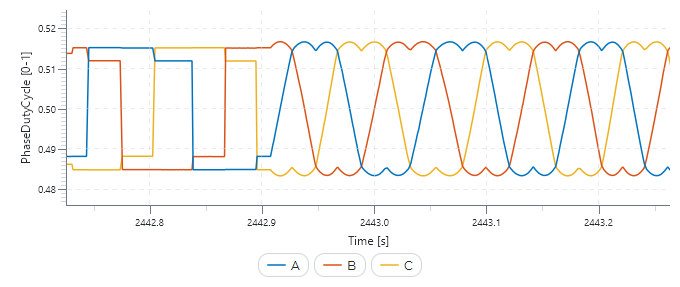
When this mode is enabled the Motor Driver will blink green (on/off) until the encoder is initialized. Once the encoder is initialized the module will change to the standard slow fading green.
Current Loop PI Gains Calculation
There is a set of "ideal" PI gains for a Discrete-Time PI Current Controller based on the motor parameters and the sampling frequency of the loop. The following implementation is derived from "A Low Cost Modular Actuator for Dynamic Robots" by Benjamin G. Katz. This math is integrated into HEBI Scope through the "Suggest Gains" button.
# CONTROLLER PARAMETERS
bandwidth = 500
i_clamp = 8.0

# CRUNCH THE NUMBERS (FROM APPENDIX OF BEN KATZ'S MASTERS THESIS)
Ts = 1 / float(sampling_frequency)
w_c = (2.0 * pi * float(bandwidth)) * Ts
kp =  R * ( (w_c) / (1 - np.exp(-R*Ts/L)) )
ki = 1 - np.exp(-R*Ts/L)