Apps and APIs
To control and use HEBI hardware we provide Applications and APIs that run on a wide variety of operating systems.
Applications
Applications include GUIs that provide a user-friendly interface for things like viewing feedback, configuring modules, or getting feedback from other devices.
| App | Description | OS Support |
|---|---|---|
A GUI for doing basic tasks on modules like visualizing feedback in real-time, manually sending commands, setting name/family, configuring controller, tuning gains, and updating firmware. |
Windows (Win64) |
|
A mobile app that provides basic user input on a touch screen and provides easy access to a number of internal sensors from the mobile device. The app provides on-screen buttons and sliders for sending digital and analog inputs, mirroring the physical capabilities of the HEBI I/O Board, that can be read in the various APIs, including a layout that acts as a joystick. |
iOS |
|
A wrapper around joysticks/gamepads that exposes inputs to the HEBI APIs as an IO-type device, and can therefore be used in place of the Mobile IO application for control inputs. |
Windows (Win64) |
APIs
APIs allow you to write programs in different languages that interface with HEBI hardware. All of these apps and APIs can be found in the Downloads section, and an a walkthrough of the core API concepts can be found here.
| API | Description | OS Support |
|---|---|---|
The Matlab API is a released API that runs in the standard Matlab working environment with no additional add-ons or toolboxes. |
Windows (Win64) |
|
The Python API is a released API that is provided as source code wrapping a C library to guarantee maximum portability across operating systems. It is available at https://pypi.python.org/pypi/hebi-py. |
Windows (Win32 / Win64) |
|
The C++ API is a released API that is provided as source code wrapping a C library to guarantee maximum portability across compilers, platforms, and operating systems. |
Windows (Win32 / Win64) |
|
We provide multiple ways of interfacing with HEBI components using both ROS 1 and ROS 2, although the ROS 1 API is legacy and no longer actively maintained. |
Linux (i686 / x86-64 / armhf / aarch64) |
|
C |
A low-level API that is generally not intended for direct use. |
Windows (Win32 / Win64) |
File Formats
HEBI uses a number of file formats to store robot configuration information in a way that is easy to version and access across the different Apps and APIs. These include kinematic information, joint-level gains, motor driver settings, and high-level robot configuration files.
| File Format | Description | Supports |
|---|---|---|
A config file format designed to store configuration information about a full system in a human-readable cross-API format. |
Scope |
|
A format that allows saving and loading of the kinematics and dynamics information about a robot configuration. |
Scope |
|
A format for saving and loading all the control parameters for the onboard controllers for individual modules, as well as groups of modules. |
Scope |
|
A format for saving and loading all the setting safety parameters (e.g. position/velocity/torque limits, m-stop strategies) for individual modules, as well as groups of modules. |
Scope |
|
A format for saving and loading all the configuration parameters for HEBI’s configurable motor driver. |
Scope |
Scope
Scope is a cross-platform graphical user interface (GUI) tool that provides configuration, monitoring, and testing capabilities for HEBI actuators and modules.
We recommend using Scope at all stages of your development, particularly its plotting and logging capabilities.
Before writing a new program Scope is useful to make sure that all devices are connected properly and that the system as a whole is working as expected. While developing and debugging a new application Scope is extremely useful for viewing the feedback and tuning gains on the live system.
Getting Started
-
Download the latest Release for your OS.
-
Make sure all modules are powered on and connected to your local network.
-
Start the application by double-clicking.
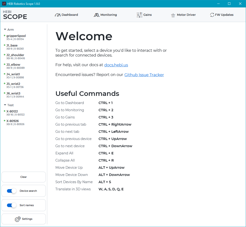
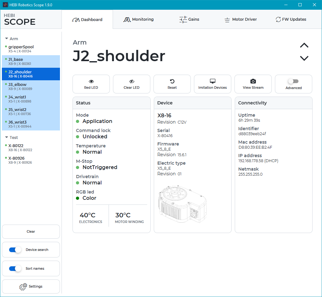
Scope starts with a screen that looks similar to the screenshot above. The items in the screenshot are, respectively:
-
A Welcome screen that provides links to the main documentation page as well as an overview of keyboard shortcuts
-
The Device Panel on the left that shows all devices visible on the network.
-
Tabs for the various panels:
-
Dashboard shows general device information such as hardware revisions and Ethernet settings, as well as various states.
-
Monitoring provides plots of device feedback as well as manual inputs for position, velocity, and effort.
-
Gains sets control strategies, gains, and safety limits.
-
Motor Driver sets parameters for motor driver devices.
-
Firmware Updates allows to safely update device firmware.
-
-
Configuration options
-
Device Search enables or disables the device lookup. Disabling will reduce network traffic, but it will keep the individual GUI elements from being updated.
-
Sort Names enables or disables the alphabetical sorting of device names. The device order can be manually modified using
ALT + UPorALT + Down -
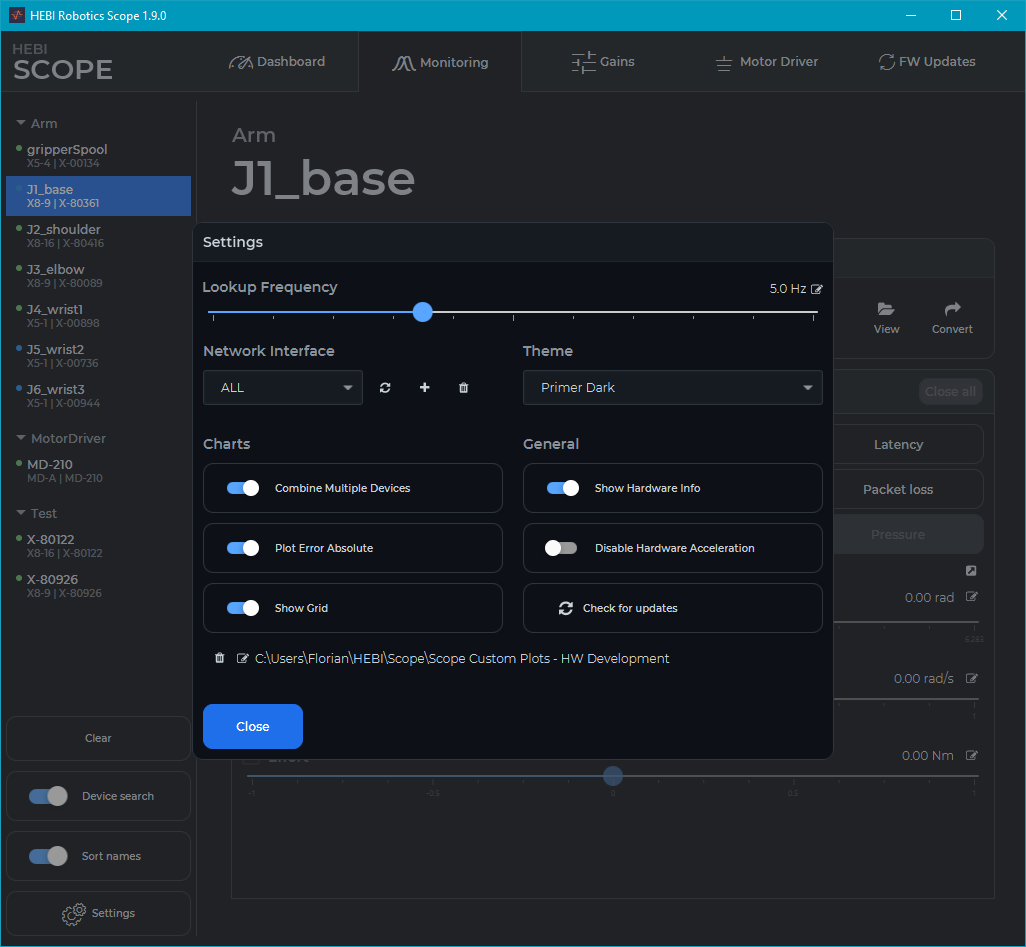
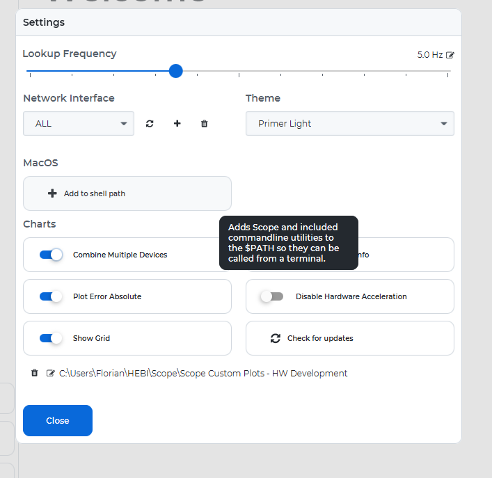
Settings: brings up a menu with additional settings as shown in the screenshot below. Please refer to the tooltips for detailed information.
-

In Settings you can also choose between different coloring themes and perform manual update checks.
Device Panel
The Device Panel shows all devices that are visible, or were recently visible, on the network.
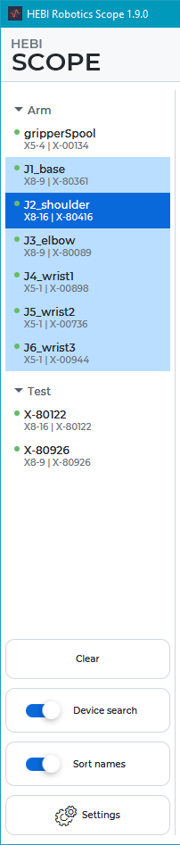
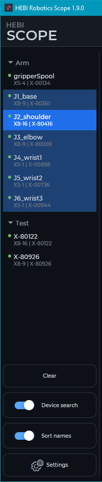
The main action in the panel is to select one or more devices for interaction. When multi-selecting, the darker highlighting represents the device that is currently in focus and corresponds to the feedback shown in the information tabs.
The colored dots indicate the current status:
-
Blue: device is reachable and in Bootloader mode
-
Green: device is reachable and in Application mode
-
Grey: device has not been reachable for at least 5 seconds
You can remove all devices that are not currently on the network (ones represented by a grey dot) by clicking the Clear button.
If you have devices that you think are currently on the network, but are not shown in the device panel, try the following:
-
Confirm that the Device Search toggle is enabled.
-
Update the network interfaces by clicking the Refresh button in the Settings Dialog.
-
Confirm that each device has successfully booted and connected to the network up by looking at the LED Status Codes
-
Confirm that the computer that Scope is running on is on the same network as the devices, and that the computer’s networks settings are properly configured.
Dashboard Tab
The Dashboard Tab shows general device information such as hardware revisions and Ethernet settings.
-
The Status section provides details of the various states that the device is in.
-
The Device section shows the details of the mechanical electrical components of the module as well as information about the currently running firmware. The mechanical details are permanent and will never change.
-
The Connectivity section shows the MAC Address of the module, which is permanent, as well as network parameters that will depend on the details of your network configuration.
-
The Advanced slider shows additional parameters that provide access to hardware features such as modifying internal encoder offsets. This should be used with caution. Refer to the tooltips for more information.
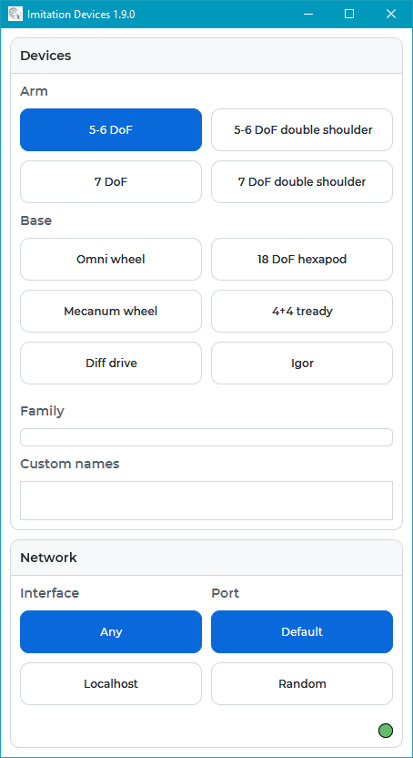
The Imitation Devices button launches a set of networked imitation modules that can be used to test and debug code before running it on real hardware. Imitation devices return commands as feedback and do not include physics feedback such as IMU data.
View Stream displays the contents of a video stream file created by hebi-video. It provides a way to view arbitrary video sources with relatively low overhead and latency.
Monitoring Tab
The Monitoring Tab provides a way to plot device feedback, work with log files, and provide basic inputs for position, velocity, and effort.
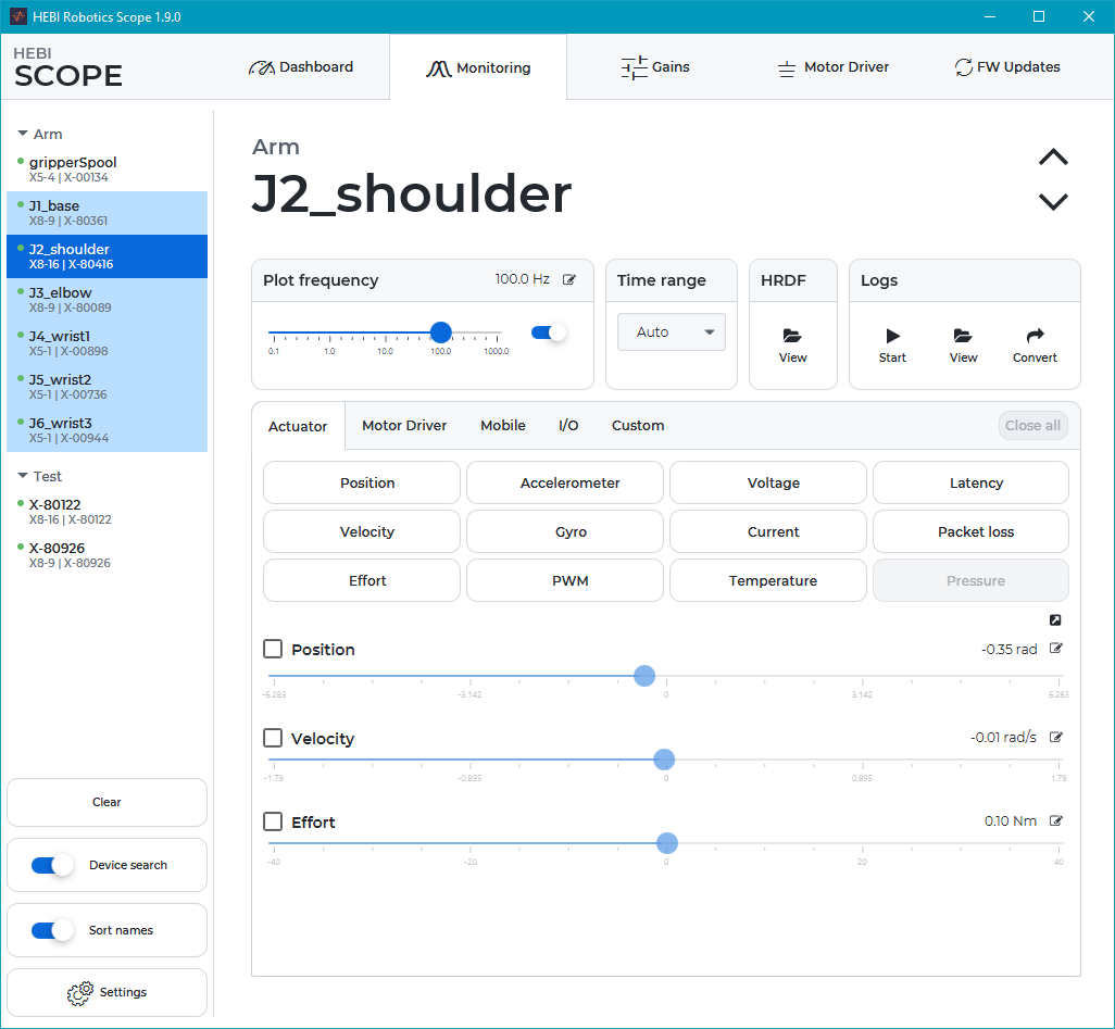
The Monitoring Tab has the following main features:
-
Plotting buttons open live charts of the selected devices at the update frequency specified by the frequency slider. The time-axis is specified by the time range, and the y-axis of charts is scaled automatically. Clicking on the legend toggles the visibility of individual traces.
-
Command sliders enable sending of basic commands to the selected modules. Commands can be any combination of position, velocity, and effort. The initial commands after enabling the slider will be set to the device’s current state. Specific values can be specified using the target buttons.
-
View HRDF creates a 3D visualization of the HRDF contents and maps the contained joints to zero or more selected devices.
-
Start Log creates a .hebilog file of the feedback of all selected modules at specified feedback frequency. Only one log can be active at a time.
-
View Log visualizes the data inside a .hebilog file.
-
Convert Log converts the contents of a .hebilog file to non-proprietary formats such as CSV or MAT.
For example, to check the position feedback from a module, select an appropriate device on the left panel, and then click Position plot to view the module’s reported position. Commands can be generated by enabling the Position checkbox and moving the corresponding slider. Alternatively, you can command an exact value using the corresponding target button.
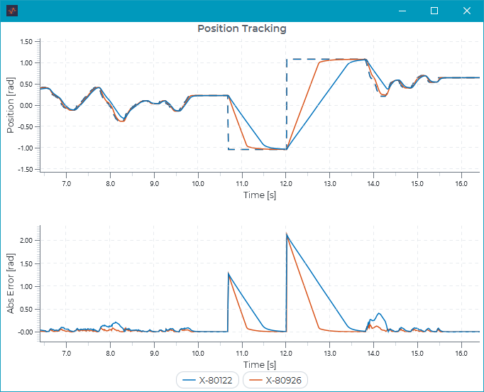
The dashed line represents the commanded position, and the solid line the feedback position.
|
Commands are sent with a command lifetime disabled. This means that commands sent from Scope to a module will stay active until another command is sent, and new commands from any API will immediately override the last command from Scope. If you close Scope, previous commands sent from Scope will still remain active on a module. Unchecking the command slider will clear a given commmand. The slider inputs will not work if someone is actively commanding an actuator with command lifetime enabled. |
Scope is a completely standalone process with a separate network connection that is independent from any user code, and can be run in parallel with any other application on the same computer or local network. When debugging your applications we highly recommend making use of Scope’s plotting capabilities in order to get live feedback on the behavior of an algorithm. For example, math errors often show up as large spikes or full drop-outs in the commanded line of position, velocity or effort.
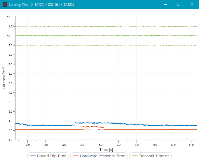
If you want to get an idea of the performance of the underlying network the Latency and Packet loss plots are useful. The image below shows a typical latency plot for a Windows 8 computer requesting feedback at 100Hz. The green dots represent the delta between received packets and provides information about the OS scheduler. The black dots represent the round-trip time of a packet going to and from a device.
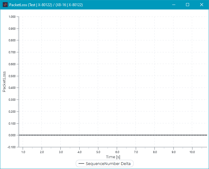
The packet loss plot should ideally show a solid line at zero. If there is frequent packet loss on a wired network (Wi-Fi is expected to have some amount of packet loss and jitter) or substantial spikes in latency there may an issue. For example:
-
Bad network connection, e.g., a network cable damaged or not plugged in correctly
-
The network is saturated, e.g., someone is copying files over the same network
-
The device is overloaded, e.g., someone is sending packets faster than a device can respond (e.g. open-loop commands from the API without pause or something else that limits the request rate)
-
The host computer is overloaded, e.g., there are too many applications running in the background
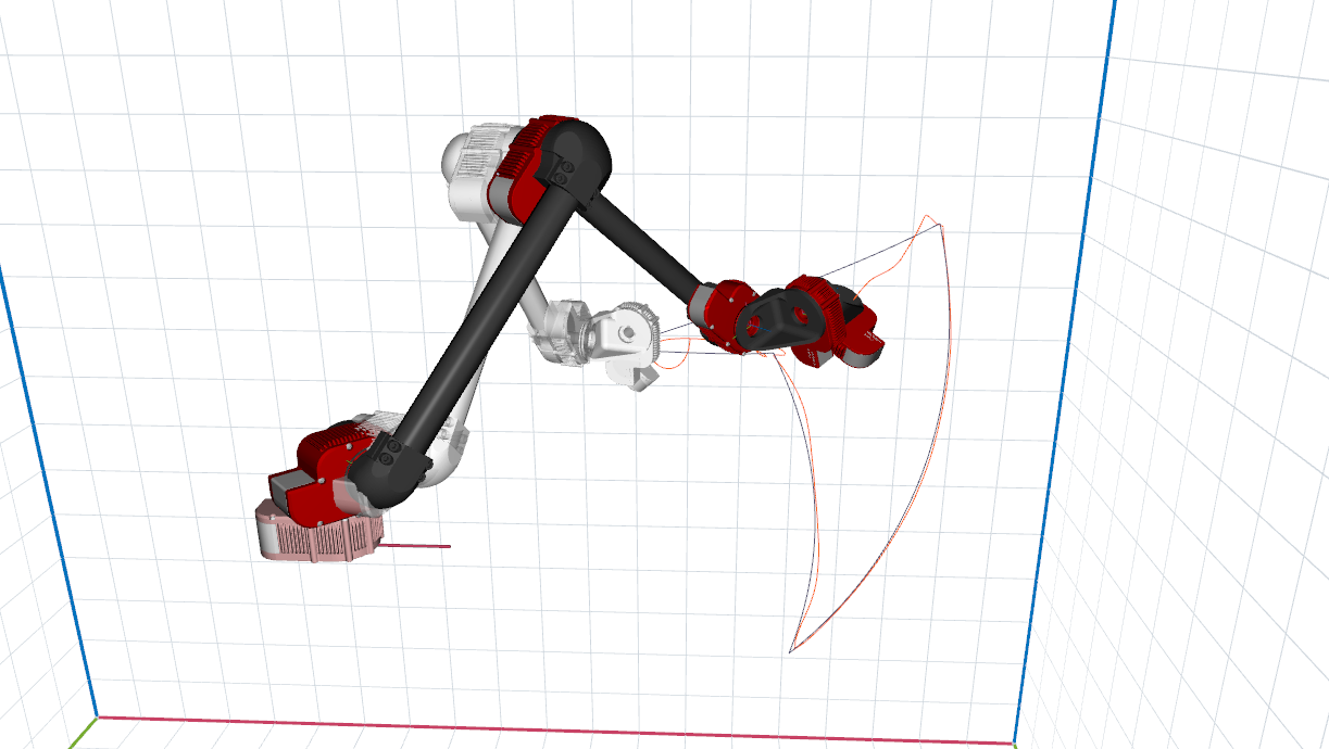
HRDF Viewer
View HRDF creates a 3D visualization of the specified .hrdf file. If devices are selected, the devices get mapped to the joints and create an online visualization of the robot configuration.
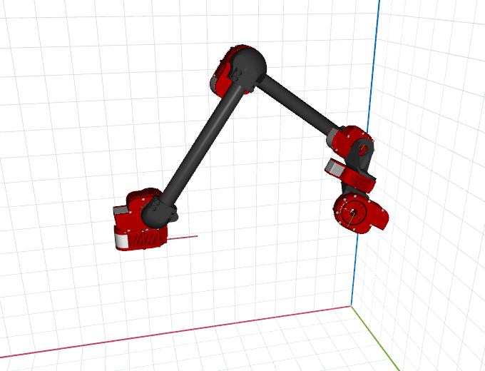
It also provides additional features such as displaying a command overlay or to orient the robot based on the first device’s IMU data. Please refer to the menu for more details.
Log Viewer
View Log opens a log viewer that shows many useful plots and provides access to the logged gains.
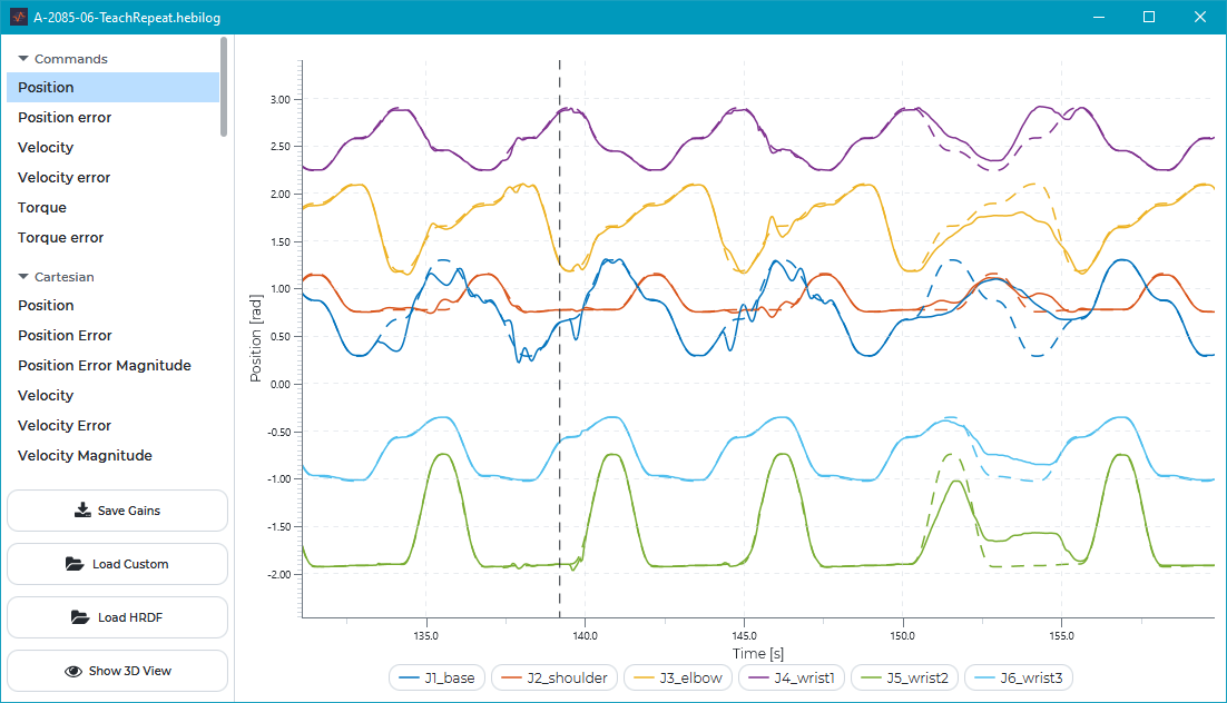
Load HRDF lets users choose a matching HRDF file to get additional charts in end-effector coordinates as well as replay the contents in a 3D visualization.
Custom Charts
It is also possible to create custom plots of feedback data. This is done by placing .XML files in the charts directory. The charts directory can be viewed and/or specified in the Settings menu.
The .XML file needs to have 2 elements, one <chart> and at least one <trace>. Valid files are loaded in alphabetical order and added as separate buttons in the Custom section of the Monitoring tab. The label that appears on the button matches the title attribute in <chart>.
<chart>
-
Attributes:
-
title: title for the button and plot header -
units: Y-Axis units -
max_samples: maximum rolling buffer size -
min_range: number, defaults to0 -
max_range: number, defaults to0 -
range_policy: behavior if trace values go out of range. Can befixedorexpanding(default).
-
-
Children:
-
<axis_x>: one or none. Defaults to a time axis -
<trace>: one or more. Each trace will be shown as a separate line.
-
<axis_x>
-
Attributes:
-
label: x axis label -
value: x values -
units: x axis units
-
<trace>
-
Attributes:
-
<label>: Name of this line in the legend -
<units>: Units -
<color>:-
red,green,blue,yellow,cyan,magenta,white,black(default), -
[0]default color for the specified index -
matlab[0]color for the specified index matching MATLAB’s default color scheme -
[x]/[y]/[z]colors used for XYZ charts,
-
-
<style>:solid(default),dashed,points -
<value>: A custom expression for calculating the current value. You have access to the latest feedback values (fbk) as well as the previous values (prevFbk). The field naming convention matches MATLAB, e.g.,fbk.positionorprevFbk.hwTxTime.
-
Examples
In custom charts you can use operators like + - * / to do basic math on different parts of module feedback. The example below creates a plot that calculates the position error, which can often be useful when tuning or evaluating the performance of a system:
<chart title="POSITION ERROR" min_range="-0.5" max_range="+0.5">
    <trace label="Position Error" units="rad" color="black" style="dashed" value="fbk.position - fbk.positionCmd" />
</chart>
The expression parser uses a Java compiler, so you may make use of math functions such as pow or sqrt. The example below calculates the magnitude of all three components of the accelerometer of a module.
<chart title="ACCEL MAGNITUDE" range_policy="fixed" min_range="0" max_range="20">
    <trace label="sqrt(x^2 + y^2 + z^2)" units="" color="black" style="solid"
           value="Math.sqrt(Math.pow(fbk.accelX,2) + Math.pow(fbk.accelY,2) + Math.pow(fbk.accelZ,2))" />
</chart>
Additional lines can be added with addititional <trace> children. You can also access the previous feedback to perform diffs over a single timestep. The example below numerically differentiates the commanded position and compares it to the commanded velocity.
<chart title="DIFF(POSITION CMD)" min_range="-3" max_range="+3" range_policy="expanding">
    <trace label="diff(positionCmd)" units="rad/s" color="black" style="points" value="(fbk.positionCmd-prevFbk.positionCmd) / (fbk.hwTxTime-prevFbk.hwTxTime)" />
	<trace label="velocityCmd" units="rad/s" color="green" style="dashed" value="fbk.velocityCmd" />
</chart>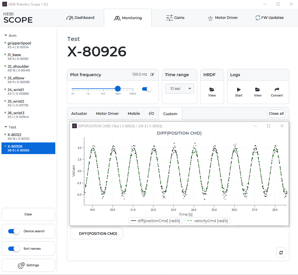
Gains Tab
The Gains Tab provides a convenient way to change control strategies, set safety limits, and to save and load gains. Tips and guidelines on tuning gains can be found in the Motion Control documentation.
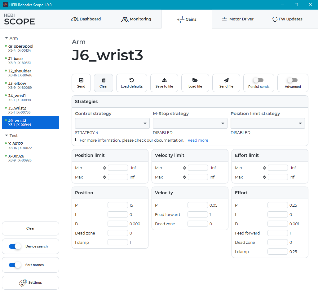
Gains can be set while a device is actively being commanded, either by Scope or from any of the APIs, by clicking at any time. This allows easy online tuning of a robot’s motion. For example, you can generate commanded positions, velocities, and efforts for an actuator programmatically (e.g. in MATLAB or C++) and use Scope to change the gains and plot the tracking performance online.
If you are commanding from Scope you will need to make sure you are not also setting the control strategy (the dropdown box is blank). In this case the command will be cleared when sending gains.
Sending gains sends all the fields shown. Empty fields are ignored. You can clear the fields by clicking the Clear button.
The default view of Gains show some of the most commonly adjusted parameters for the position, velocity, effort controllers on an actuator. The full list of parameters can be viewed by toggling the Show Advanced switch. Details on all of these parameters can be found in the Motion Control documentation.
|
Gains are non-persisting parameters. This means that they will be reset to the last saved (persisted) values on reboot. To ensure that the current values are restored at next boot, you can enable the "Persist Sends" toggle or click |
Saving/Loading Gain files
Gains can be saved in a group-compatible gain format by selecting one or more devices and pressing the save to file button. The gains of multiple devices will be stored in the same order as they appear on the device pane.
Load file reads a gain file and loads the values into the corresponding input fields. Only one set of gains can be displayed at a single time.
Send File loads the gains of an arbitrary number of modules and immediately sends them to the selected devices, without populating the input fields. The order will again match the order in the device pane.
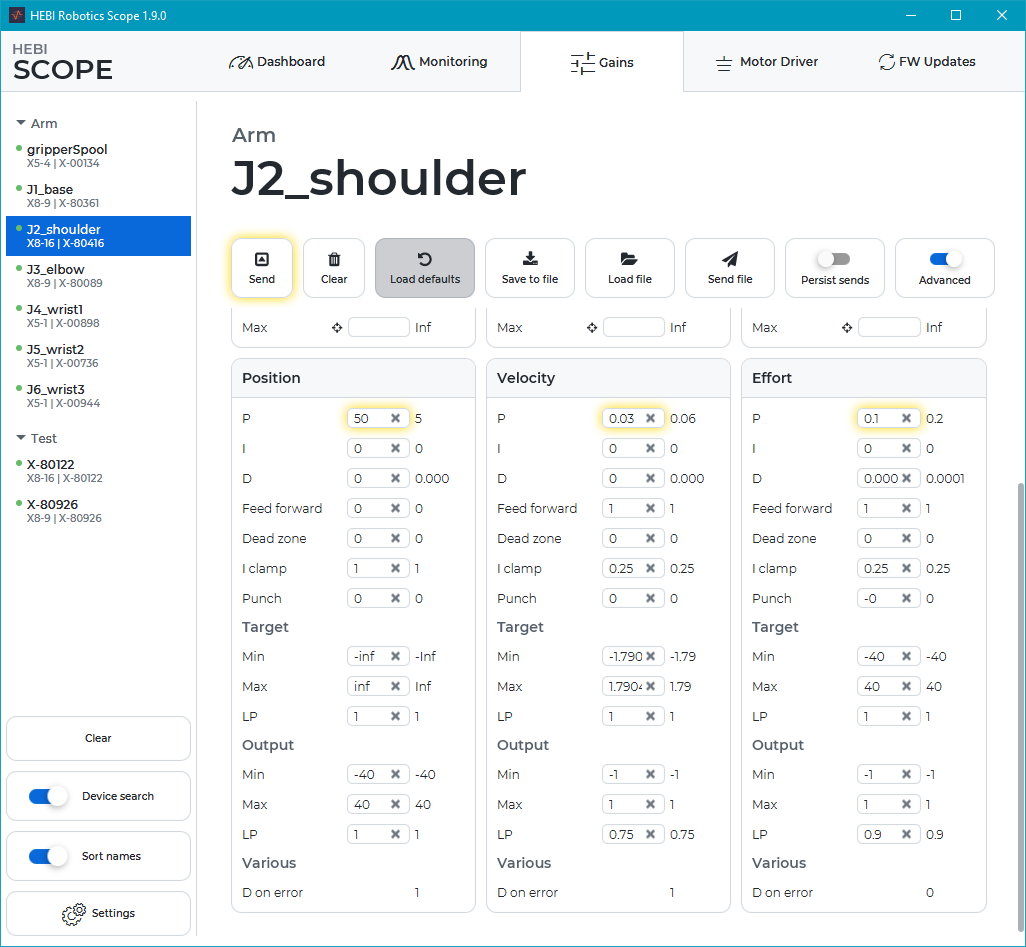
Resetting Gains
In many cases it is useful to reset or compare the active gains to the default values for an actuator. An easy way to do this is by using Load Defaults, which downloads the appropriate default gains for the selected hardware type and control strategy. Differences compared to the active gains are highlighted in yellow.
|
Loading the default gains for a module requires an active internet connection. For cases that do not have access to the internet, we provide downloadable default gains that can be stored and loaded offline. |
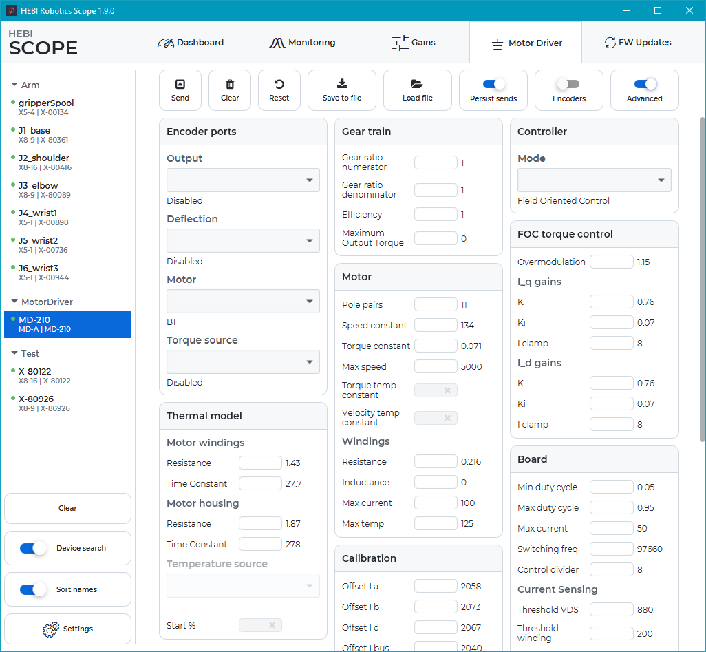
Motor Driver Tab
The motor driver tab provides control of parameters related to turning a custom encoder and motor into a HEBI compatible actuator. Please refer to the built-in tooltips for more information on the individual fields.
Updating Firmware
HEBI releases updates to the internal device firmware that contain performance improvements, additional features, and bugfixes. Each device has an isolated Bootloader mode, so updates can be done safely without the risk of disabling a module. You can check for updates using the Refresh button. Updating firmware requires an internet connection.
We strive to maintain backwards and forwards compatibility in firmware udpates. In the rare cases where we do break backwards compatibility, we will send out email notifications to all customers. If you have any concerns about a firmware update, please check the Firmware Changelog or email us at support@hebirobotics.com.
|
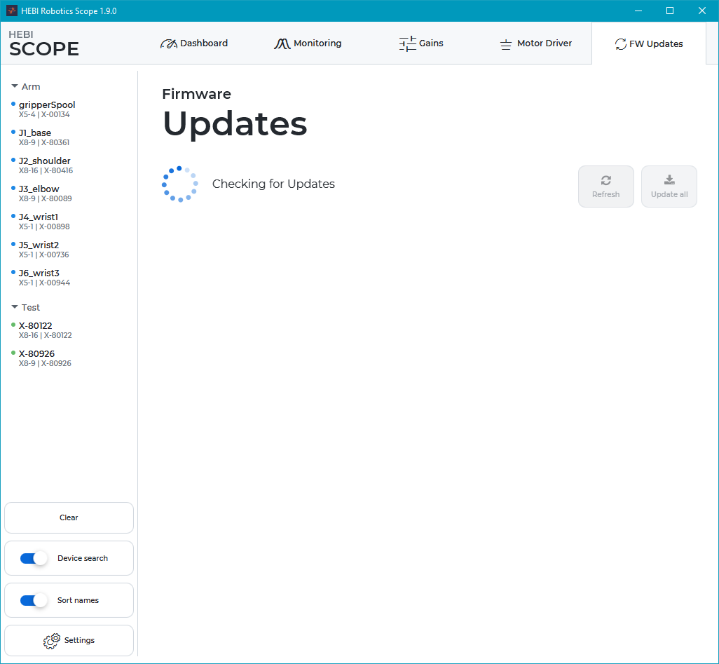
The refresh will show all modules for which updates are available. You can then update individual devices, or all of them at once. The devices will automatically reboot into Bootloader, download the appropriate application firmware, and reboot.
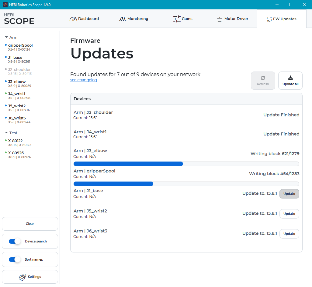
Updating a device should take about 10 seconds. Cancelling or interrupting an update will not "brick" the module, but may require you to run the update process again.
Scope CLI
Scope ships with an additional command line interface (CLI) that provides useful file loading and configuration utilities without requiring the graphical interface. On Windows and Linux the command line tools are installed automatically. On macOS you need to click Add to shell path in the macOS specific settings.
hebi-config
The hebi-config tool can send configuration files to specified devices. Calling hebi-config --help prints a detailed list of all available parameters.
For example, sending a motor driver configuration to a named device looks like this
hebi-config --name MD-210 --motor-driver path/to/MD-210.xml --persist --resetMultiple entries can be added multiple times or in comma separated lists
hebi-config --name J1_base --name J2_shoulder --names J3_elbow,J4_wrist1,J5_wrist2, J6_wrist3 --gains path/to/arm_gains.xmlhebi-gateway-server & -client
It is sometimes desired to connect to devices on a remote network through tunnels or VPNs. Broadcasts are generally limited to the local network, so we developed a Gateway connection that can forward local lookup requests to remote networks. With this feature, if computer 1 is running the gateway, a secondary computer 2 can connect to and interact with the devices located on computer 1’s network as if they were local to computer 2.
There are two utilities, hebi-gateway-server and hebi-gateway-client that serve two different use cases.
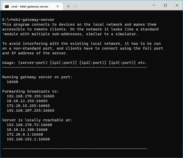
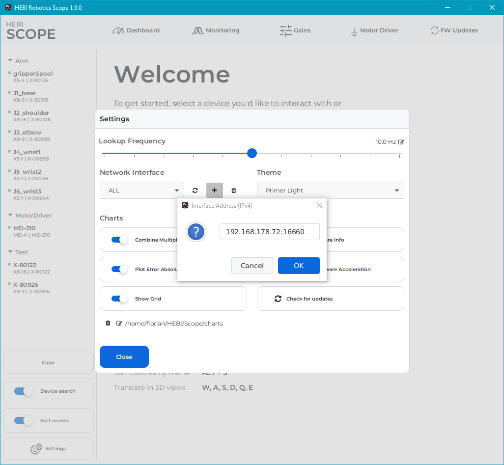
The hebi-gateway-server connects to one or more unicast or broadcast ip addresses and exposes all discovered devices on the server port (defaults to 16660). In a VPN scenario, this application would run on the remote network and allow remote lookups.
The tool prints out a Server is locally reachable at section that lists all the available addresses of the remote host.
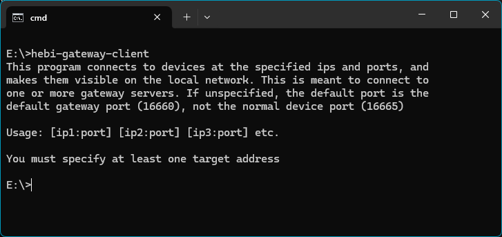
The hebi-gateway-client connects to one or more addresses (port 16660) and exposes found devices on the default device port, where they can be seen by lookups with the default settings.
In the VPN scenario, this application would run on the local network and connect to one of the lookupAddresses shown in the hebi-gateway-server. However, note that the client is functionally equivalent to manually adding the remote addresses to Scope or the APIs, so it is not technically required.
In case you are not familiar with setting up VPNs, we recommend taking a look at ZeroTier. It can setup a private network with bi-directional communications between multiple individual computers across the Internet.
Multiple HEBI device emulation apps on one host
Some of our applications, e.g., imitation groups or simulator devices, emulate a physical device interface that needs to listen on the default udp port in order to be found by Scope or API lookups. Due to port limitations, each port may only be bound to one application.
If you for some reason need to run multiple emulator apps, e.g., imitation and a joystick interface, you can run them on different ports and combine them using hebi-gateway-client.
For example, you can select custom port 2800 in the imitation device interface, and run hebi-gateway-client 127.0.0.1:2800.
WSL2 Gateway
Windows Subsystem for Linux v2 (WSL2) lets Windows users run a GNU/Linux environment that is very tightly integrated with the host OS. While the Linux versions of the HEBI APIs and tools can run without modification, the environment runs inside a virtual machine that is on a separate network and prevents any devices from being seen.
Until WSL2 adds features to expose raw network interfaces, this limitation can be worked around by (1) launching the VPN Gateway on the Windows side,
# run on Windows
hebi-gateway-server
and subsequently (2) adding the shown IP address on the WSL2 Linux side.
| Scope with basic plotting capability can be run using X-forwarding. For setup instructions please refer to How to set up working X11 forwarding on WSL2. |
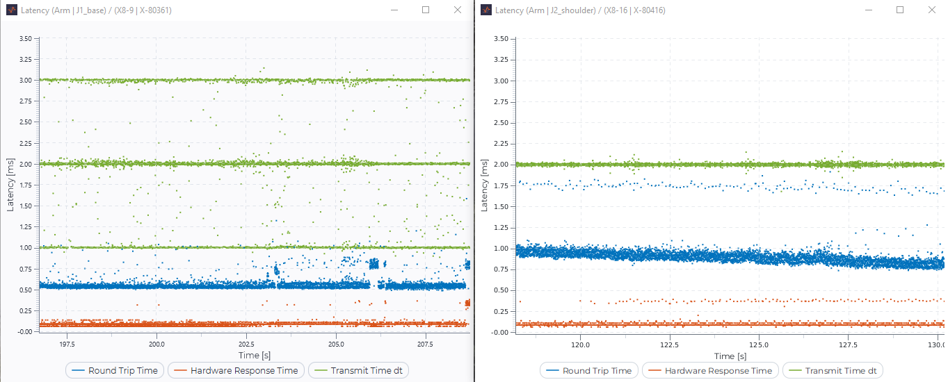
When you run code on WSL2 you can expect the frequency to track significantly better (green dots) at the cost of slightly higher latency (blue dots) due to the additional indirection. The charts below show latency plots running simultaneously on the same computer on Windows (left) and Ubuntu 20.04 on WSL2 (right):
hebi-video
The video acquisition tool for Scope’s video stream viewer is packaged as a separate app due to size concerns. You can download the latest release.
| Downloading the HEBI Video .exe application from the link above will install all of the files required to run the commands below from your OS command terminal. |
Video streams can be acquired from different sources, including Webcams, IP-cameras, or video files. The stream acquisition updates a memory mapped file, which can simultaneously be viewed in Scope and be opened in an API. Streams can be restarted or changed at any time and do not crash the viewer.
Below are some examples for different sources:
# Syntax
openStream {outputFile} {source} ({width} {height} {fps})

# First USB camera on Windows at 1920p resolution
openStream usb0.stream 0 1920

# Streaming an input file
openStream file.stream recordedVideo.mp4

# Stream from an IP-camera using rtsp
openStream ipcam.stream rtsp://${user}:${pw}@${ip}/stream0
The acquisition is configured to prefer low latency over saving computation time or reducing artifacts. openStream is based on bundled versions of FFMpeg and OpenCV, and is using software decoding.
The package also bundles a GStreamer based OpenGStreamerStream with support for hardware decoding for improved latency. Depending on your system you may need to install the GStreamer library (see instructions).
# Stream from an IP-camera using rtsp w/ possible hardware decoding
OpenGStreamerStream ipcam.stream rtsp://${user}:${pw}@${ip}/stream0
Using hebi-video with the HEBI CR1 Camera Module
HEBI Camera Modules use RTSP to stream the camera feed over the network connection. In order to visualize the camera stream, determine the IP Address of the RPi in the Camera Module through Scope as shown below.
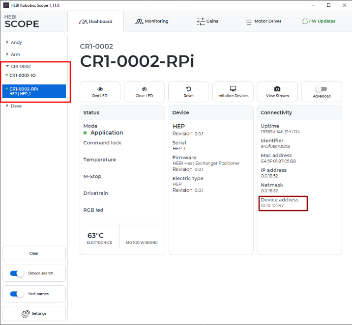
Once you have located the RPi IP Address, use it with the following command:
# Stream from a HEBI RPi Camera Module
openStream CR1.stream rtsp://{ip}:8554/test
# Example with IP shown above
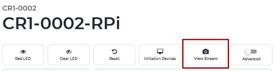
openStream CR1.stream rtsp://10.10.10.247:8554/testRunning this command will generate a .stream file that scope can use to view the stream with the View Stream button.
Charts API
We provide a programmatic API for Scope-like 2D and 3D visualizations. For detailed documentation, please refer to the hebi-charts-examples repository.

Mobile I/O
HEBI Mobile I/O is a free app for iOS and Android that provides a way of using a mobile device to generate general-purpose input/output in the HEBI APIs. Its main feature is a touch-screen interface that mimics a game-controller layout and provides digital and analog feedback in the same format that you would read from the HEBI I/O Board. The app also exposes internal sensors, including the mobile device’s IMU, magnetometer, GPS-based location data, and on compatible devices it provides the estimated 6-DoF pose of the device using ARKit in iOS and ARCore in Android.
Getting Started
-
Get the app for free from:
-
Make sure the mobile device is connected to your local network.
-
Launch the app.
-
In order to get pose feedback based on ARKit/ARCore, you will have to allow the app to access the device camera. This is because ARKit uses the camera to track features in the world to estimate the devices full 6-DoF pose.
-
-
Access feedback from the mobile device in Scope or any of the APIs.
-
Matlab Examples (Github)
-
Python Examples (coming soon)
-
C++ Examples (coming soon)
-
App Settings
In both Android and recent iOS versions, the name and family of the mobile device can be set using Scope by right-clicking the mobile device on the left side panel, or by setting the name and family from any of the APIs.
Android
There are also switches in the app to enable/disable GPS location feedback and ARCore pose feedback.
iOS
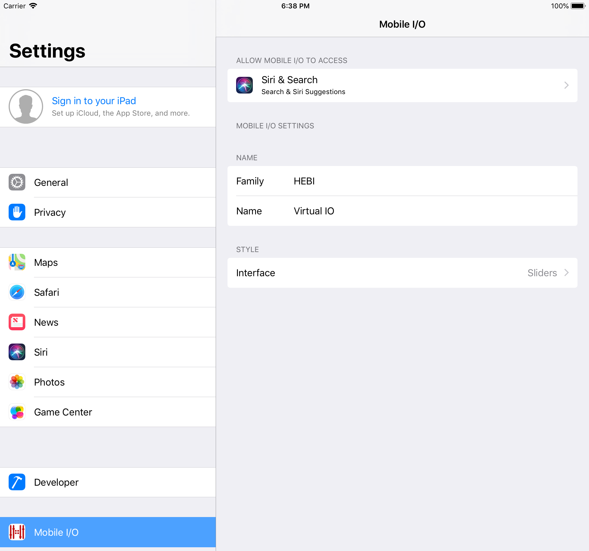
In iOS the name and family of the mobile device can be set in the settings panel for the app, found going to iOS Settings, and scrolling down the app list until you see Mobile I/O. This name and family will be how the device appears in Scope and the APIs. You can also change the layout of the iOS app to an alternative portrait Sliders view, instead of the default landscape Joystick layout. Finally, you can select whether or not the acceleration feedback that is returned from the application includes the acceleration due to gravity, or filters this information out.
Joystick View
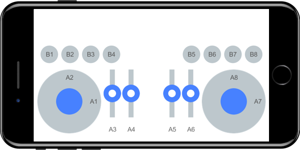
The joystick layout of the app provides 8 buttons and up to 8 analog sliders or joystick axes that you can use for input. The way the APIs communicate input from these buttons and axes are detailed in the table below. The buttons and axes are labeled on the screen. Note that the layout of the buttons and sliders may differ depending on the device.
Device Feedback
Overall, the API provides access to feedback from a mobile device the same way it does for other HEBI modules. Its main feature is a touch-screen interface that mimics a game-controller layout and provides digital and analog feedback in the same format that you would read from the HEBI I/O Board.
The Mobile I/O app also returns other sensor data, including the full 6-DoF pose of the device calculated using ARKit / ARCore on supported. The feedback availability, accuracy, and precision will depend on the device and operating system. 3
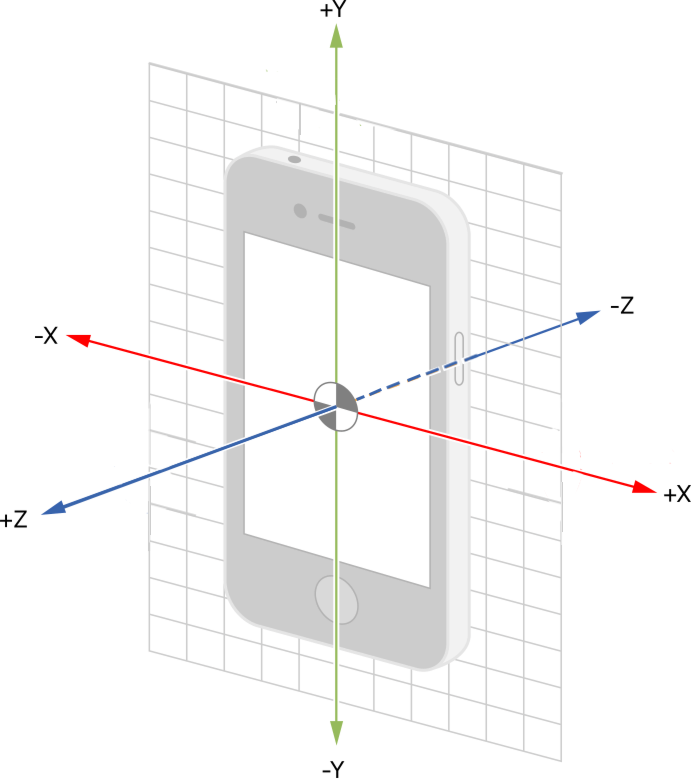
Reference Frame
Where applicable, the reference frame for the feedback from the device follows the convention of the iOS Core Motion framework (see image below).
I/O Feedback
| Parameter | Units | Description |
|---|---|---|
|
|
The current time from the system clock used by the API. This is a single value that corresponds to all feedback at this timestep. |
|
|
The system time when feedback was received by the device. The most recent of these times is what is reported as the single |
|
|
The system time when feedback requests were sent to the device. |
|
|
The hardware timestamp when the device transmitted its feedback. Time initializes at 0 when the app is launched. |
|
|
The hardware timestamp when the device received a request for feedback. Time initializes at 0 when the app is launched. |
|
|
8 analog inputs based on touch input from joysticks or sliders in the app. |
|
|
8 digital inputs based on touch input from buttons in the app. |
Mobile Feedback
| Parameter | Units | Description |
|---|---|---|
|
|
The current time from the system clock used by the API. This is a single value that corresponds to all feedback at this timestep. |
|
|
The system time when feedback was received by the decice. The most recent of these times is what is reported as the single |
|
|
The system time when feedback requests were sent to the device. |
|
|
The hardware timestamp when the device transmitted its feedback. Time initializes at 0 when the app is launched. |
|
|
The hardware timestamp when the device received a request for feedback. Time initializes at 0 when the app is launched. |
|
|
The device’s estimated linear 3-DoF acceleration from an internal IMU, excluding gravitional acceleration. Depending on the API, XYZ values are combined together into a single vector or returned individually. |
|
|
The device’s sensed 3-DoF angular velocity from an internal IMU. Depending on the API, XYZ values are combined together into a single vector or returned individually. |
|
|
The device’s sensed 3-DoF magnetic field from an internal magnetometer. Depending on the API, XYZ values are combined together into a single vector or returned individually. |
|
|
Altitude reported by the device barometer. Not yet supported. |
|
|
The device’s 3-DoF orientation, based on Core Motion in iOS and the equivalent motion sensor APIs in Android. Depending on the API, quaternion components are combined together into a single vector or returned individually. |
|
|
Latitude position on the surface of the earth, as reported by the device location services, which includes GPS. Currently Android only. |
|
|
Longitude position on the surface of the earth, as reported by the device location services, which includes GPS. Currently Android only. |
|
|
Altitude above sea level, as reported by the device location services, which includes GPS. Currently Android only. |
|
|
The bearing of the horizontal direction of travel of this device, based from true north. Currently Android only. |
|
|
The standard deviation of the uncertainty of the horizontal lat/long position of the device. Currently Android only. |
|
|
The standard deviation of the uncertainty of the vertical altitude of the device. Currently Android only. |
|
|
The GPS time when feedback was received for GPS-related feedback. Currently Android only. |
|
|
The device’s orientation in the world, based on ARKit / ARCore. Depending on the API, quaternion components are combined together into a single vector or returned individually. |
|
|
The device’s position in the world, based on ARKit / ARCore. Depending on the API, position components are combined together into a single vector or returned individually. |
|
|
Status of the tracking from ARKit / ARCore.
The values listed here are used for Scope and the Matlab API. In other APIs they are an |
|
|
Charge level of the device’s battery (in percent). |
Info Feedback
| Parameter | Units | Description |
|---|---|---|
|
|
The current user-settable name that a device shows up as in a |
|
|
The current user-settable family that a device shows up as in a |
|
|
A unique identifier of the device, displayed in the format of a MAC address. This is not the actual MAC address of the device. |
|
|
The IP Address of the device. |
|
|
The network mask of the device. |
|
|
The gateway of the device. |
|
|
The unique identifier of the device provided by iOS. |
|
|
The class of device, e.g. |
|
|
The specific revision of the device, e.g. |
|
|
The operating system of the device, e.g. |
|
|
The version of the operating system, e.g. |
|
|
The name of the app. |
|
|
The version of the app. |
Device Commands
The Mobile I/O applications also can be configured by and display/react to commands sent from Scope or the APIs.
I/O Commands
| Parameter | Units | Description |
|---|---|---|
|
|
Sets the "snap to" location for a joystick axis (default 0) or slider (default disabled). Sending |
|
|
Sets the button behavior to momentary (default, 0) or toggle (1). The toggle state is identified by white text on the button, whereas the momentary state is black. |
|
|
Illuminates (1) or hides (0) a indicator ring around the corresponding button. |
|
|
If a joystick axis or slider is not in "snap" mode, and is not actively being moved, then this moves the joystick axis or slider to the given location. For joystick commands that are out of the unit circle range, this projects the desired point back to the unit circle. |
General Commands
| Parameter | Units | Description |
|---|---|---|
|
|
Sets the color of a border around the outside perimeter of the app |
|
|
For non-zero commanded values, causes the app to vibrate momentarily (on supported devices) |
HEBI Input
The HEBI Input program is a small python script that runs on computer, exposing the inputs of a connected joystick or gamepad as a HEBI IO board device. In this way, you can use the Mobile IO wrapping classes available in the HEBI APIs to access and react to the joystick controls in the same way as using the Mobile IO app as an input device.
Note that this cannot be run at the same time from the same computer as the "imitation group" feature within Scope, as these bind to the same network port.
Getting Started
-
Download the zip from here:
-
HEBI Input (.zip)
-
-
Extract into a local directory
-
Install the dependent packages by running
python3 -m pip install -r requirements.txt -
Modify the
keymap.ymlto match the input events for the joystick/gamepad you are using; this mapping may vary depending on the host OS. We provide a keymap for the Voyee XBox clone gamepad. -
Run
-
Mac/linux:
./controller_mobile_io.py --key_config <controller yaml file> --family <DesiredFamilyName> -
Windows:
python3 controller_mobile_io.py --key_config <controller yaml file> --family <DesiredFamilyName>
-
The joystick should now be visible to devices on the same network through Scope; you can view the feedback in real time by going to the "I/O" sub-tab of the "monitoring" tab.
You can pass the --name parameter to adjust the initial name, or the --port parameter to change the default port that is used (e.g., to use multiple instances simultaneously in conjunction with the hebi-gateway-client tool).
You can view all the command line options for the current version by running python3 controller_mobile_io.py -h
Device Feedback
Overall, the API provides access to feedback from the HEBI input script in the same way it does for other HEBI modules. The primary benefit is providing an interface to the joystick without requiring code changes on the control software side or any third-party libraries. The feedback is exposed in the same format that you would read from the HEBI I/O Board.
HEBI APIs
HEBI provides libraries and programmatic APIs that enable users to control complex systems in real-time directly from MATLAB, Python, or C. These APIs are designed to have parallel features, although syntax varies slightly between language. The flexibility allows the user to work in the environment they are most comfortable with and which matches the system requirements. For example, MATLAB and Python can be used for fast prototyping and testing of algorithms on real hardware without the need for compilation and code generation; both are fast and powerful enough for delivering a final software solution. Alternatively, C can be used to compile an application to run with a small footprint within a deployed linux system.
MATLAB
MATLAB is a proprietary scripting language and computing environment developed by Mathworks. It is widely used for data analysis and research across many engineering disciplines. The language’s focus on linear algebra and matrix operations makes it a very good language for programming robots.
| We currently do not officially support Simulink. For more details, please refer to the Simulink Support thread on the forums. |
Python
Python is an easy-to-learn, powerful general purpose programming language with broad package support that makes it useful for beginners as well as for advanced applications.
C++
C++ is a powerful, general purpose advanced programming language. It has a steeper learning curve than Python or MATLAB, but allows the software engineer more control over aspects such as memory management.
Quick Links
-
MATLAB
-
Python
-
C++
-
API 2.4 (.zip)
-
Examples (GitHub)
-
Issue Tracker (Github)
-
Python Package (PyPI)
-
API Examples (GitHub)
-
API 3.16.0 (.zip)
-
API 3.16.0 (.tar.gz; preserves symlinks for macOS/Linux shared libraries)
-
API Documentation (Doxygen)
-
Examples (GitHub)
Also available are earlier versions of the API and Doxygen documentation.
The examples are divided into a few folders: basic, advanced, and kits. The basic examples are designed as a hands-on tutorial for getting started with the API; we highly recommend downloading and going through these examples as concrete/runnable examples of the concepts discussed in this documentation.
|
Installation/Project Integration
-
MATLAB
-
Python
-
C++
| The HEBI API for MATLAB requires MATLAB R2013b or newer. |
First, download the latest Release and extract the contents into a directory of your choice. Then, open MATLAB and add the "hebi" directory to the search path.
The path can be added manually by right-clicking on the directory,
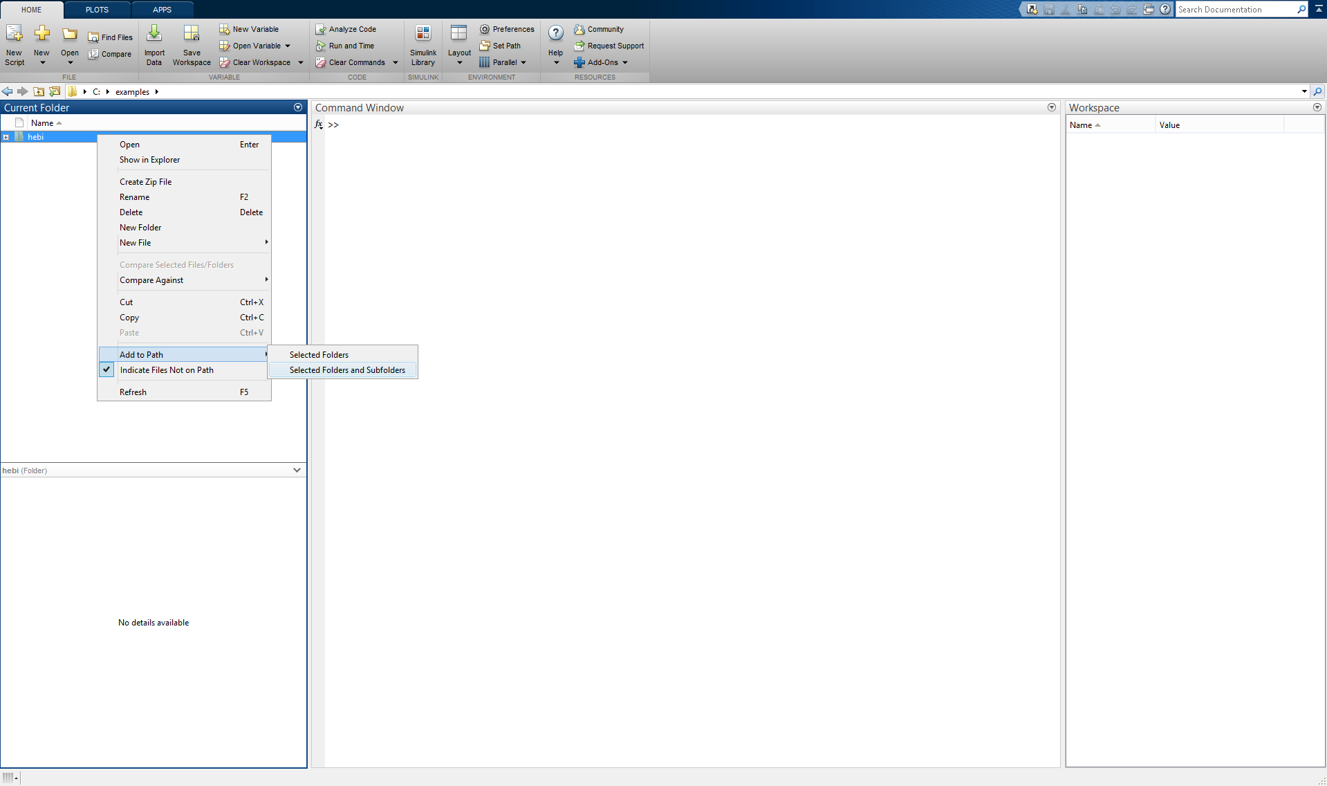
or programmatically by calling the built-in addpath function.
addpath([pwd '/hebi']);For incorporating the HEBI library into a project, we recommend creating a startup script that can add the necessary files automatically.
function [] = startup()
% startup sets up libraries and should be started once on startup.
currentDir = fileparts(mfilename('fullpath'));
addpath(fullfile(currentDir , 'hebi'));
hebi_load(); % explicitely pre-load library
end
It is usually a good idea to increase MATLAB’s Java Heap Size using the slider control panel in Preferences→General→Java Heap Memory. In particular this will allow larger .hebilog files to be loaded into memory.
|
NOTE: As of hebi-py version 2.0.0, only Python 3 is supported. You must use a hebi-py version 1.x.y
for Python 2 compatibility.
The HEBI Python API is available through PyPI, which requires the use of pip.
The API requires numpy, which is available on practically any platform Python 3 is supported.
For some functions in the hebi.util module, matplotlib is required; however,
matplotlib is not a hard requirement since it may not be available on machines without a graphical user interface (e.g., a Linux machine without an X server).
It is recommended to install matplotlib through your package managers on most Linux distros.
Matplotlib’s website documentation elaborates more on specific dependencies and how to compile from source.
|
While not a requirement for the HEBI Python API itself, some of the kit examples (e.g., igor) also require some SDL libraries:
The GitHub examples repository provides the SDL2 library for Windows users.
It is automatically loaded when necessary on Windows, but not for Linux and
MacOS. Linux and MacOS users must install it themselves. Debian/Ubuntu
users can install it using sudo apt-get install libsdl2-2.0-0 and Fedora/RHEL
users can install it using sudo [yum|dnf] install SDL2.
|
Installing from the command line
From the command line, you can download the API from pip:
# On Linux, it is recommended to install to the user directory
pip install --user hebi-py
# Other platforms (e.g., Windows, MacOS)
pip install hebi-py
Installing from IDEs
Most modern IDEs (e.g., PyCharm) have pip integration by default.
You can use the provided facilities to find the hebi-py package and install it.
Remarks
Some Linux distributions prefer you to install numpy through their package manager.
For example, Ubuntu uses the package python3-numpy; Red Hat/CentOS/Fedora use python3-numpy.
For some Linux environments, you may not be able to easily install matplotlib because
you do not have a desktop environment (e.g., running a server Linux install on a Raspberry Pi).
For such environments, you cannot use the plotting functions under hebi.util, but the rest
of the API will not be affected.
The C++ API is made up of:
-
The
.cppand.hppfiles that comprise the source code of the C++ wrapper around the underlying C library. -
The
hebi.hheader file that provides the function declarations for the underlying C library. -
The actual dynamic/shared object library that must be linked into your program (
.dllfor Windows,.sofor Linux, and.dylibfor macOS).
| The C++ API is designed to be used with the C++ 11 standard; when building your project, ensure you have set the proper compiler switches to enable this support (e.g., -std=c++11 for gcc). |
There are a few basic ways to integrate the API into your program:
-
If you are using Visual Studio, use the NuGet package manager to add the HEBI C++ API as a dependency. You will have to disable "precompiled header" support for the API to properly compile with your project.
-
Use the examples as a template for setting up a CMake or Visual Studio project dependent on the C++ API.
-
Add the source
.cppfiles to your project sources, ensure your include path contains the.hppandhebi.hfile, and link in the shared object for your platform and architecture.
Device Discovery
The HEBI APIs provide an easy to use facility to discover and communicate with HEBI modules on network interfaces. The HEBI Lookup class encapsulates a background process that automatically discovers HEBI devices on the local network using UDP broadcast messages.
The default settings of the Lookup object should be appropriate for most users, but are configurable.
-
MATLAB
-
Python
-
C++
The first call to HebiLookup initializes the background discovery process
HebiLookupThe default settings may be changed in hebi_config.m.
This Lookup class acts as a singleton, but can be disposed of after creating the desired Group objects.
import hebi
lookup = hebi.Lookup()
Generally, you will only need one hebi::Lookup object per application, and it can be disposed of after creating the desired hebi::Group objects (see Device Selection).
#include "lookup.hpp"

int main() {
  // Create Lookup
  hebi::Lookup lookup;
  // Do stuff...
  return 0;
}
The default settings may be changed by calling functions on the hebi::Lookup object.
Displaying the Lookup object provides an overview of all devices that are visible on the network. The Family and Name fields/columns show the user-settable names.
-
MATLAB
-
Python
-
C++
Here the Serial Number field/column shows the unique serial number of each device as well.
% explicit display
disp(HebiLookup);

% implicit display (no semicolon)
HebiLookup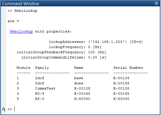
To view the modules that have been discovered, use the EntryList class to programmatically access the contents at a snapshot in time.
The entries also have fields such as IP address and MAC address, and whether or not the module is "stale" (no longer responding to requests from the Lookup object).
import hebi
from time import sleep
lookup = hebi.Lookup()
# Give the Lookup process 2 seconds to populate entries
sleep(2)
print('Modules found on network:')
for entry in lookup.entrylist:
  print(f'{entry.family} | {entry.name}')
Depending on the available modules, the output will look similar to
Modules found on network:
Arm | J1_base
Arm | J2_shoulder
Arm | J2_elbow
Base | left_wheel
Base | right_wheel
To view the modules that the Lookup has discovered, use the hebi::LookupEntry class to programmatically access the contents at a snapshot in time.
The entries also have fields such as IP address and MAC address, and whether or not the module is "stale" (no longer responding to requests from the Lookup object).
// Create Lookup and wait for it to populate
hebi::Lookup lookup;
std::this_thread::sleep_for(std::chrono::seconds(2));

// Take snapshot and print to the screen
auto entry_list = lookup.getEntryList();
std::cout << "Modules found on network:" << std::endl;
for (auto entry : entry_list)
{
  std::cout << entry.family_ << " | " << entry.name_ << std::endl;
}
Depending on the available modules, the output will look similar to:
Modules found on network:
Arm | J1_base
Arm | J2_shoulder
Arm | J2_elbow
Base | left_wheel
Base | right_wheel
In case you need programmatic access to other details (e.g. ip address, mechanical type, etc.) of all devices, you can use the group interface.
-
MATLAB
-
Python
-
C++
% form a group of all devices
devices = HebiLookup.newGroupFromFamily('*');
infoTable = devices.getInfo();
lookup = hebi.Lookup()
# form a group of all devices
devices = lookup.get_group_from_family('*')
info = devices.request_info()Some fields (such as Ethernet Info, Firmware Version Info, UserData, Runtime Data, aren’t included by default to reduce network traffic, and can be requested with the request_info_extra function:
// retrieve info
info = devices.request_info_extra()
hebi::Lookup lookup;
std::this_thread::sleep_for(std::chrono::seconds(2));
// form a group of all devices
auto group = lookup.getGroupFromFamily("*");
// retrieve info
GroupInfo group_info(group->size());
bool success = group->requestInfo(&group_info);Some fields aren’t included by default due to their size, and can be requested with the requestInfoExtra hebi::Group function:
// retrieve info
bool success = group->requestInfoExtra(&group_info, InfoExtraFields::EthernetInfo | InfoExtraFields::FirmwareInfo);
(see the enum documentation for the InfoExtraFields linked from the requestInfoExtra function. Note that you can bitwise-or these enums to retrieve multiple, such As
static_cast<InfoExtraFields>(InfoExtraFields::EthernetInfo | InfoExtraFields::FirmwareInfo))
Note the info request can fail (throw an error in MATLAB, return None in Python, and return false in C++) if devices are 'stale' (haven’t responded in several seconds) in which case stale devices would have to be cleared first:
-
MATLAB
-
Python
-
C++
% reset everything to the initial state
HebiLookup.initialize()

% rebuild only the device table
HebiLookup.clearModuleList();
pause(0.5); % allow time to re-buildlookup.reset()lookup.reset()If for some reason devices are not listed, please refer to the following troubleshooting table.
| Problem | Suggestions |
|---|---|
A device fails to get an IP address (LED fades orange / green) |
|
A device did successfully get an IP address (e.g. LED fades green), but is not visible in the lookup |
|
The lookup does not initialize to the default settings (MATLAB) |
|
If you encounter an issue connecting to devices that was not covered in the table above, please contact us directly.
Joint-Level Control
Device Selection
The Lookup object can create a Group instance. A group is a collection of modules (often part of the same robotic system), and the group interface represents the basic way to send commands and retrieve feedback. They provide convenient ways to deal with modules and handle high-level issues such as data synchronization and logging. Modules can be identified by user settable parameters, such as name or family, or hardware constants, such as their serial number or mac address.
-
MATLAB
-
Python
-
C++
A HebiGroup can be created from HebiLookup in different ways:
% Creating a group by selecting custom names
family = 'leg';
names = {'hip', 'knee'};
group = HebiLookup.newGroupFromNames(family, names);
% Can provide a different family for each module
families = {'mobile_base', 'mobile_base', 'arm', 'arm'};
names = {'left_wheel', 'right_wheel', 'shoulder', 'elbow'};
group = HebiLookup.newGroupFromNames(families, names);% Creating a group by selecting constant serial numbers
serials = {
'X-00134'
'X-00148' };
group = HebiLookup.newGroupFromSerialNumbers(serials);% Providing '*' as the family selects all modules
devices = HebiLookup.newGroupFromFamily('*');A comprehensive list of all available calls for selecting devices can be found in the HebiLookup API.
A Group can be created from HebiLookup in different ways:
# Create a group from a set of names
group = lookup.get_group_from_names(['leg'], ['hip', 'knee'])
# Can provide a different family for each module
families = ['mobile_base', 'mobile_base', 'arm', 'arm']
names = ['left_wheel', 'right_wheel', 'shoulder', 'elbow']
group = lookup.get_group_from_names(families, names)# Providing '*' as the family selects all modules
group = lookup.get_group_from_family('*')The Lookup class documentation provides a comprehensive set of functions used to create group objects.
A hebi::Group can be created from HebiLookup in different ways:
// Create a group from a set of names
std::shared_ptr<Group> group = lookup.getGroupFromNames({"leg"}, {"hip", "knee"});
// Can provide a different family for each module
std::vector<std::string> families = {"mobile_base", "mobile_base", "arm", "arm"};
std::vector<std::string> names = {"left_wheel", "right_wheel", "shoulder", "elbow"};
std::shared_ptr<Group> group = lookup.getGroupFromNames(families, names);// providing "*" as the family selects all modules
std::shared_ptr<Group> group = lookup.getGroupFromFamily("*");The Lookup class documentation provides a comprehensive set of functions used to create group objects.
| The example names and serial numbers need to be modified to match devices that were found on your network during the discovery step. |
| If you do not have access to physical devices, you can still test the API or control algorithms using the Imitation Device feature in Scope. |
Commands
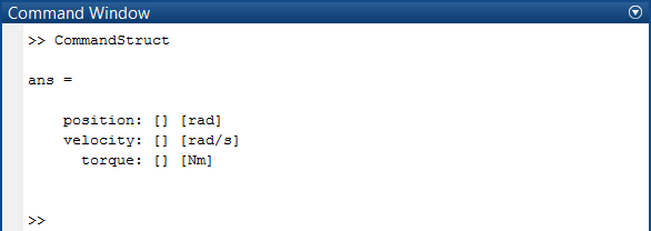
Position, velocity, torque (effort), and many other fields can be commanded by using the Command API functions. A CommandStruct (MATLAB) or GroupCommand object (Python/C++) are used to store the commands to be sent to the group.
-
MATLAB
-
Python
-
C++
Position, velocity, and torque (effort) can be commanded by using a CommandStruct.
Each field expects a 1xN vector where N is the number of devices within a group. Leaving a field empty or setting a value within a vector to NaN corresponds to turning the corresponding control loop off.
% Send a zero force/effort command to a group with two actuators
cmd = CommandStruct();
cmd.effort = [0 0];
group.send(cmd); % immediately sends messages to all grouped devices
A GroupCommand object
is used to store the commands to be sent to the group with the group.send_command() function.
We use types from the numpy library
to update many of the fields with vectors of data.
# numpy is aliased to np throughout this documentation.
import numpy as np
import hebi

# Create a numpy array filled with zeros
efforts = np.zeros(group.size)

# Command all modules in a group with this zero force or effort command
group_command = hebi.GroupCommand(group.size)
group_command.effort = efforts
group.send_command(group_command)
The command affects the actuator control loops only if at least one of the position, velocity, and effort command fields is not cleared.
In particular, a command sent with all three of these cleared will not affect the control loop setpoints.
However, if only a subset of the fields are set (e.g., only position), then commands from the other fields will be cancelled when this message is receieved.
If you want to completely cancel out a previous command (especially when the Command Lifetime is not set!) and turn the control loops off,
you can set the commanded value to nan.
|
A few ways to get a nan in Python are:
# parse from string
a = float('nan')
# numpy provides it as an attribute
b = np.nan
The individual Command elements of a
GroupCommand
object can also be
accessed and updated individually. Note that you cannot create an instance of
Command - you only retrieve references through a
GroupCommand.
The Command object provides the same interface as a GroupCommand, but with
all of the fields returning a scalar as opposed to a vector or matrix.
As an example, updating the name of the module in the following example:
import hebi
group_command = hebi.GroupCommand(group.size)
command = group_command[0] # Retrieve reference to the command for first module
command.name = "new name"
# Only changes the name for the first module
group.send_command_with_acknowledgement(group_command)
A hebi::GroupCommand object is used to store the commands to be sent to the group. We use types from the open-source C++ matrix library Eigen to update many of the fields with vectors of data.
// Create an Eigen vector object filled with zeros
Eigen::VectorXd efforts(group->size());
efforts->setZero();

// Command all modules in a group with this zero force or effort command
hebi::GroupCommand group_command(group->size());
group_command.setEffort(efforts);
group->sendCommand(group_command);
The command affects the actuator control loops only if at least one of the position, velocity, and effort command fields is not cleared.
In particular, a command sent with all three of these cleared will not affect the control loop setpoints.
However, if only a subset of the fields are set (e.g., only position), then commands from the other fields will be cancelled when this message is receieved.
If you want to completely cancel out a previous command (especially when the Command Lifetime is not set!) and turn the control loops off,
you can set the commanded value to NAN (see std::numeric_limits::quiet_NaN).
|
The individual hebi::Command elements of a GroupCommand object can also be accessed and updated individually. Note that you cannot create an instance of Command - you only retrieve references through a GroupCommand. The hebi::Command object provides a hierarchical message that provides access to all of the available options that can be sent through the API — for example, updating the name of the module in the following example:
hebi::GroupCommand group_command(group->size());
hebi::Command& command = group_command[0]; // retrieve reference to command for first module
command.settings().name().set("new name");
bool success = group->sendCommandWithAcknowledgement(group_command);
The Command class documentation provides complete documentation of the Command class fields.
Setting the values in the CommandStruct/GroupCommand object does not affect/command any modules until the command is sent to the group.
|
| Individual commands only set the low-level controller targets for the current instant in time, and do not calculate a trajectory from the current state to the desired target state. In other words, setting a single position command will result in a step response from the actuator. If you’d like a smooth motion between two or more positions, please take a look at the Trajectory API. |
Command Lifetime
Commands are only valid for a limited command lifetime, so even unchanging setpoints need to be re-sent before they expire. This means that is a script or process is killed (e.g., with ctrl-c), commanded motions are aborted. By default, the command lifetime is 250ms.
-
MATLAB
-
Python
-
C++
This is set on a per-group basic via the CommandLifeTime function.
% Set command lifetime to 100ms
group.setCommandLifetime(0.1);
% Self commands in a loop to continue
cmd = CommandStruct();
while true
    cmd.position = [0 0];
    group.send(cmd); % immediately sends messages to all grouped devices
    pause(0.01);
end
This is set on a per-group basis with the Group.command_lifetime field.
# Sets command timeout to 100 milliseconds
group.command_lifetime = 100.0
# Command must be sent in loop at a faster rate than the lifetime in order to remain in effect.
while not stop_loop:
  group.send_command(group_command)
  sleep(0.01)
This is set on a per-group basis with the hebi::Group::setCommandLifetimeMs() function.
Note that this function will return 'false' if
attempting to set a value longer than the maximum allowable command lifetime.
// Sets command timeout to 100 milliseconds
group->setCommandLifetimeMs(100);
// Command must be sent in loop at a faster rate than the lifetime in order to remain in effect.
while (!stop_loop)
{
  group->sendCommand(group_command);
  std::this_thread::sleep_for(std::chrono::milliseconds(10));
}
Example Use Cases
The following example shows an open-loop controller commanding sine waves with different frequencies on two actuators using simultaneous position and velocity control.
-
MATLAB
-
Python
-
C++
% Two actuators executing sine waves of 1Hz and 2Hz
group = HebiLookup.newGroupFromNames('leg', {'knee', 'ankle'});
cmd = CommandStruct();
w = 2 * pi * [1 2];
t0 = tic();
while true
    t = toc(t0);
    cmd.position = sin( w * t );
    cmd.velocity = cos( w * t ) * w;
    group.send(cmd);
    pause(0.001);
end
% Two actuators executing sine waves of 1Hz and 2Hz
group = lookup.get_group_from_names(["leg"], ["knee", "ankle"])
group.command_lifetime = 20.0
group_command = hebi.GroupCommand(group.size)
w = np.array([math.pi*2.0, math.pi*4.0], dtype=np.float64)
w_t = np.empty(2, dtype=np.float64)
t = 0.0
dt = 0.01 # 10 ms
while not stop_loop:
np.multiply(w, t, w_t)
group_command.position = np.cos(w_t)
group_command.velocity = np.sin(w_t)
group.send_command(group_command)
sleep(dt)
t = t + dt#include <cmath> // provides M_PI
...
// Two actuators executing sine waves of 1Hz and 2Hz
auto group = lookup.getGroupFromNames({"knee", "ankle"}, {"leg"});
group->setCommandLifetimeMs(20);
hebi::GroupCommand group_command(group->size());
Eigen::VectorXd w
<< 2.0 * M_PI,
4.0 * M_PI;
// It is good practice not to allocate this every loop iteration.
Eigen::VectorXd w_t(2);
double t = 0.0;
double dt = 0.01; // 10 ms
while (!stop_loop) {
w_t = w * t;
group_command.setPosition(w_t.array().cos());
group_command.setVelocity(w_t.array().sin());
group->sendCommand(group_command);
std::this_thread::sleep_for(std::chrono::milliseconds(dt * 1000.0));
t += dt;
}Note in addition to actuator commands such as position, velocity, and effort, we can also command values for other types of modules. Here, we set the value on an I/O board digital output pin to 'high'.
-
MATLAB
-
Python
-
C++
The IoCommandStruct serves as a similar structure to command the outputs on an I/O board. Note that for I/O boards we found it to be more maintainable to create a mapping and to access the individual pin fields by string as shown below.
% Pin mapping
led_r = 'c6';

% Turn on red LED
group = HebiLookup.newGroupFromNames('IO_BOARD', 'sensor interface');
cmd = IoCommandStruct();
cmd.(led_r) = 1;
group.send(cmd);
group = lookup.get_group_from_names(["IO_BOARD"], ["sensor interface"])
group_command = hebi.GroupCommand(group.size)
group_command.io.c.set_int(6, 1) # set IO pin "c6" to 1 for every module in group
group.send_command(group_command)auto group = lookup.getGroupFromNames({"IO_BOARD"}, {"sensor interface"});
hebi::GroupCommand group_command(group->size());
group_command[0].io().c().setInt(6, 1); // Set IO pin "c6" to 1 for the first module in the group
group->sendCommand(group_command);Delivery Acknowledgement
Commands can be dropped on particularly poor or congested networks, and the Group "send" functions do not provide guaranteed delivery or even an acknowledgement of receipt; they are designed for relatively high-frequency applications where commands are resent frequently (e.g. 100Hz).
For commands that are only sent once (such as setting gains on the modules), we recommend using the send command with acknowledgement functions to provide positive confirmation that the command was received.
-
MATLAB
-
Python
-
C++
When sending a command, adding 'RequestAck' requests message acknowledgements from each
device, and will return true if acknowledgements have been received from all devices
within this group and within the specified timeout.
send
success = group.send(cmd, 'RequestAck', true);(also, see the HebiUtils.sendWithRetry example in the Gains section below)
See the Group.send_command_with_acknowledgement function.
success = group.send_command_with_acknowledgement(group_command)Use Group::sendCommandWithAcknowledgement to verify the command was received.
success = group->sendCommandWithAcknowledgement(group_command);Other Commands
The Group API "send" methods additionally supports various other commands such as programmatically setting names, resetting devices, setting safety limits, and setting LED colors. LEDs can for example be used to provide live feedback to people standing next to a robot, or for synchronizing/debugging motions in combination with a high-speed camera.
-
MATLAB
-
Python
-
C++
LEDs and other commands can be sent with the send method.
group.send('led', 'red'); % set all to red
group.send('led', [0 0 1]); % set all to blue [r g b] [0-1]
group.send('led', []); % reset to default mode
You can override the LED color on each individual module.
# Set all to red
color = hebi.Color(255, 0, 0) // red, green, blue
group_command = GroupCommand(group.size)
group_command.led.color = color
# This is equivalent:
# group_command.led.color = 'red'
group.send_command(group_command)-
and allow the module to reclaim control over the color.
# Set all to be module controlled
# This is the default mode
group_command = GroupCommand(group.size)
group_command.led.color = 'transparent'
group.send_command(group_command)
You can override the LED color on each individual module.
// Set all to red
hebi::Color color(255, 0, 0); // red, green, blue
hebi::GroupCommand groupCommand(group->size());
for (int i = 0; i < group->size(); i++) {
	groupCommand[i].led().setOverrideColor(color);
}
group->sendCommand(groupCommand);-
and allow the module to reclaim control over the color.
// Set all to be module controlled
// This is the default mode
hebi::GroupCommand groupCommand(group->size());
for (int i = 0; i < group->size(); i++) {
	groupCommand[i].led().setModuleControl();
}
group->sendCommand(groupCommand);
Feedback
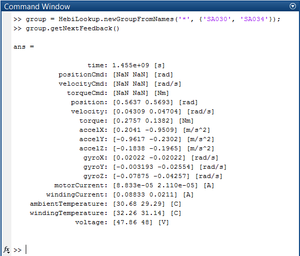
Each group continuously gathers sensor feedback from all contained devices in a background thread, and synchronizes the data into a single struct. This loop rate of this background thread is the Group’s feedback_frequency, which defaults to 100Hz and is configurable on a per-group basis. A group can asynchronously access the received feedback with the "get next feedback" function. Note that each call returns the next new (not previously accessed) synchronized feedback. Thus, a single feedback response will never be returned more than once. If there is no new feedback since the last call to this function, it will block and wait for a new packet (up to a configurable timeout), so this can be used as an easy way to control the rate of a loop. For example:
-
MATLAB
-
Python
-
C++
Call getNextFeedback to return the next feedback, and to change the default rate call setFeedbackFrequency or modify the hebi_config.m file.
% This effectively sets the rate of the loop below to (a maximum of) 200Hz
group.setFeedbackFrequency(200.0)

while running
  fbk = group.getNextFeedback()
end
Our devices tend to return a large number of sensors, so we have added different 'views' in order to enable advanced use cases without confusing new users. The default view returns feedback of the most used types of sensors, but there are alternative views in case you’d like to access additional information such as hardware timestamp data.
% Basic feedback (position, velocity, effort (e.g. torque), IMU data, temperature)
fbk = group.getNextFeedback();

% Advanced feedback including hardware timestamps
fbk = group.getNextFeedbackFull();

% I/O board feedback
ioFbk = group.getNextFeedbackIO();

% Mobile device feedback including location services and AR features
mobileFbk = group.getNextFeedbackMobile();
Call Group.get_next_feedback to return the next feedback, and set Group.feedback_frequency to change the default rate. Feedback is returned as a GroupFeedback object.
# Best practice is to allocate this once, not every loop iteration
group_feedback = hebi.GroupFeedback(group.size)

# This effectively sets the rate of the loop below to (a maximum of) 200Hz
group.feedback_frequency = 200.0

while not stop_loop:
  if group.get_next_feedback(reuse_fbk=group_feedback) is None:
    continue

  # ... read/use feedback object contents here.
The GroupFeedback object contains position, velocity, and effort actuator feedback, as well as sensor feedback from a number of sensors. Similar to commands, many of the values can be accessed as numpy vectors or matrices, with one row for each module in the group.
# Fill in feedback
group_feedback = hebi.GroupFeedback(group.size)
group_feedback = group.get_next_feedback(reuse_fbk=group_feedback)

# Retrieve positions:
positions = group_feedback.position
print(f'Position Feedback:\n{positions}')

# Get Gyro
gyros = group_feedback.gyro
print(f'Gyro Feedback:\n{gyros}')

# Individually access io pin feedback from first module
io_a = group_feedback.io.a
if (io_a.has(1)):
  print(f'PinA: {io_a.get_int(1)[0]}')
Call getNextFeedback() on the Group to return the next feedback, and call Group::setFeedbackFrequencyHz to change the default rate.
Feedback is returned as a Group Feedback object.
// Best practice is to allocate this once, not every loop iteration
hebi::GroupFeedback feedback(group->size());

// This effectively sets the rate of the loop below to (a maximum of) 200Hz
group->setFeedbackFrequencyHz(200);

while (!stop_loop)
{
  if (!group->getNextFeedback(&feedback))
    continue;
  // ... read/use feedback object contents here.
}
The GroupFeedback object contains position, velocity, and effort actuator feedback, as well as sensor feedback from a number of sensors. Similar to commands, many of the values can be accessed as Eigen vectors or matrices, with one row for each module in the group. Fields can also be accessed via individual hebi::Feedback object references, which allow hierarchical access to all information contained in the feedback message.
// Fill in feedback
hebi::GroupFeedback group_feedback(group->size());
group->getNextFeedback(&group_feedback);

// Retrieve positions:
Eigen::VectorXd positions = group_feedback.getPosition();
std::cout << "Position feedback: " << std::endl << positions << std::endl;

// Update an existing Eigen vector or matrix (eliminates a copy operation)
Eigen::MatrixX3d gyros(group->size());
group_feedback.getGyro(gyros);
std::cout << "Gyro feedback: " << std::endl << gyros << std::endl;

// Individually access io pin feedback from first module
auto& io_a = group_feedback[0].io().a();
if (io_a.has(1))
std::cout << "Pin A1: " << io_a.get(1) << std::endl;| The actual feedback frequency is fundamentally limited by the underlying operating system’s scheduler. For example, code that executes at a rate of 1KHz in Linux may be limited to ~640Hz on Windows 7. For typical rates below 250Hz this tends to be irrelevant. The Importance of Metrics and Operating Systems contains more information about the expected performance for various operating systems. |
| Feedback from multiple devices is typically synchronized to within 1ms. However, the actual timings depends on the network layout and external network traffic. Please see Analyzing the viability of Ethernet and UDP for robot control for more information. |
Other Methods to Return Feedback
In Python and C++, there are two other approaches to return feedback from a group that may be appropriate for some use cases. The first is a callback-based approach, where the background thread that is synchronizing feedback from individual modules invokes the callback each time a new synchronized GroupFeedback is available. To use this method, use the API to add a feedback handler with the designated function signature:
-
MATLAB
-
Python
-
C++
The callback-based approach is not compatible with the MATLAB API.
# Function feedback callback
def feedback_func_callback(feedback):
  # feedback is guaranteed to be a "hebi.GroupFeedback" instance
  # ... read/use feedback object contents here

# Sets frequency to 200 Hz
group.feedback_frequency = 200.0

# Add feedback handler
group.add_feedback_handler(feedback_func_callback)
The C++ 11 std::function will automatically convert function pointers and lambda functions to a function object. The callback will execute on a background thread. Below we show two methods for adding a callback function
// Function feedback callback
static void feedback_func_callback(const hebi::GroupFeedback& const feedback) {
  // ... read/use feedback object contents here
}

void foo() {
  // Sets frequency to 200 Hz
  group->setFeedbackFrequencyHz(200);

  // Method 1: Add pointer to function
  group->addFeedbackHandler(feedback_func_callback);

  // Method 2: Add a lambda function; see C++ reference for more info
  group->addFeedbackHandler(
      [](const hebi::GroupFeedback& const feedback) -> void {
        // ... read/use feedback object contents here
      }
  );
}
The second method allows finer grained control over the network traffic that is sent. You can retrieve feedback when the feedback frequency is zero by manually sending a feedback request.
-
MATLAB
-
Python
-
C++
The "send individual request" approach is not compatible with the MATLAB API.
group_feedback = hebi.GroupFeedback(group.size)
# Sends a request to the modules for feedback and immediately returns
group.send_feedback_request()
# Blocks until feedback is in the background queue or timeout
group_feedback = group.get_next_feedback(reuse_fbk=group_feedback)
hebi::GroupFeedback feedback(group->size());
// Sends a request to the modules for feedback and immediately returns
group->sendFeedbackRequest();
// Blocks until feedback is in the background queue or timeout
group->getNextFeedback(&feedback);
Setting the feedback frequency on the group effectively calls the send feedback request function at a certain rate on a background thread.
|
Closed-Loop Control Example
The below example shows a closed-loop controller that implements a virtual spring that controls torque (effort) to drive the output towards the origin (stiffness = 1 Nm / rad).
-
MATLAB
-
Python
-
C++
% Virtual spring on single device
group = HebiLookup.newGroupFromNames('HEBI', 'J1');
cmd = CommandStruct();
stiffness = 1; % [Nm/rad]
while true
    fbk = group.getNextFeedback();
    cmd.effort = -stiffness * fbk.position;
    group.send(cmd);
end
import hebi
# Virtual spring
lookup = hebi.Lookup()
# change to your name(s)/family(s)
group = lookup.get_group_from_names(["HEBI"], ["J1"])
command = hebi.GroupCommand(group.size)
stiffness = 1.0 # [Nm/rad]
feedback = hebi.GroupFeedback(group.size)
while not stop_loop:
# wait for the feedback
if group.get_next_feedback(reuse_fbk=feedback) is None:
continue
command.effort = feedback.position * -stiffness
group.send_command(command)Using a lambda callback, this can be rewritten as:
import hebi

# Virtual spring
lookup = hebi.Lookup()
# change to your name(s)/family(s)
group = lookup.get_group_from_names(["HEBI"], ["J1"])
command = hebi.GroupCommand(group.size)
stiffness = 1.0 # [Nm/rad]

def fbk_handler(feedback):
  command.effort = feedback.position * -stiffness
  group.send_command(command)

group.add_feedback_handler(fbk_handler)
// Virtual spring
hebi::Lookup lookup;
auto group = lookup.getGroupFromNames({"HEBI"}, {"J1"}); // change to your name(s)/family(s)
hebi::GroupCommand command(group->size());
hebi::GroupFeedback feedback(group->size());
const double stiffness = 1.0; // [Nm/rad]
while (!stop_loop) {
if (!group->getNextFeedback(&feedback)) // wait for the feedback
continue;
command.setEffort(-stiffness * feedback.getPosition());
group->sendCommand(command);
}Using a lambda callback, this can be rewritten as:
// Virtual spring
hebi::Lookup lookup;
auto group = lookup.getGroupFromNames({"HEBI"}, {"J1"}); // change to your name(s)/family(s)
hebi::GroupCommand command(group->size());

const double stiffness = 1.0; // [Nm/rad]

while (!stop_loop) {
  // Add callback, capturing relevant variables by reference and/or value
  [&group, &command, stiffness](const hebi::GroupFeedback& const feedback) -> void {
    command.setEffort(-stiffness * feedback.getPosition());
    group->sendCommand(command);
  }
}
Performance and Efficiency
The API has been developed with low latency and high efficiency in mind. For applications that require high control frequencies, we recommend the following additional steps.
-
MATLAB
-
Python
-
C++
-
Reuse command structs rather than allocate one each time in a loop
% Don't allocate CommandStruct in a loop
cmd = CommandStruct();
while true
    cmd.position = desiredPosition;
end-
Reuse feedback structs by passing an existing struct into getNextFeedback
% Create feedback struct once and reuse it
tmpFbk = group.getNextFeedback();
while true
    fbk = group.getNextFeedback(tmpFbk);
end-
Use convenience wrappers instead of passing parameters where possible
% Parameterized
fbk = group.getNextFeedback('view', 'full');

% Convenience wrapper (recommended)
fbk = group.getNextFeedbackFull();-
Decrease the frequency of minor garbage collections by increasing the new space in the java.opts file. Note that this is useful for applications that need to run for extended periods of time (e.g. days/weeks) and is overkill for 99.9% of applications. It may also negatively impact e.g. live plotting.
# Minimum total heap
-Xms4g

# Maximum total heap
-Xmx4g

# Young generation heap space
-Xmn3g-
Reuse Command and Feedback objects rather than allocating one each time in a loop
# Best practice is to allocate this once, not every loop iteration
group_feedback = hebi.GroupFeedback(group.size)
group_command = hebi.GroupCommand(group.size)
pos = np.zeros(group.size, dtype=np.float64)

while not stop_loop:
    # wait for the feedback
    if group.get_next_feedback(reuse_fbk=group_feedback) is None:
        continue

    # edit "pos"
    ...
    # set command data
    group_command.position = pos
group.send_command(group_command)-
Our benchmarking and empirical tests have shown that for normal use of our API, even to control complex time-critical systems like (e.g., our Igor kit at 200Hz), the above basic optimization results in code that does not run into performance limitations on most systems. There is enough spare overhead that even calling the most expensive calls (kinematics related calls) on the order of 1kHz you should not run into issues. However, for some applications such as running on slower embedded systems (e.g., Raspberry Pi) or pre-planning and sampling motions (such as a collision-validation step on the motion of an arm), the marshalling of the data to and from the underlying C API may add enough overhead to limit performance. In these cases, porting code to use the C++ API may provide a performance boost.
-
Reuse Command, Feedback and Eigen objects rather than allocating one each time in a loop
// allocate groupCommand outside tight loop below
hebi::GroupCommand groupCommand(group->size());
hebi::GroupFeedback group_feedback(group->size());
Eigen::VectorXd posVector = Eigen::VectorXd::Zero(group->size());

while(!stop_loop) {
  // wait for the feedback
  if (!group->getNextFeedback(&group_feedback))
    continue;
  // edit "posVector"
  ...
  // set command data
  groupCommand.setPosition(posVector);
  group->sendCommand(groupCommand);
}-
If using vectorized access to group feedback fields, pass in an existing Eigen object rather than returning a new one
hebi::GroupFeedback group_feedback(group->size());
Eigen::VectorXd positions(group->size());
if (group->getNextFeedback(&group_feedback)) {
  // Prefer passing in reference rather than returning copy
  group_feedback.getPosition(positions);
}
Gains
The gains of the control loops executed on each device can be programmatically read and written. The recommended way to set and load gains is to use the XML Gains Format that works across HEBI APIs and GUI tools. These files can then be edited using a standard text editor.
We generally recommend explicitly setting the gains at the start of each script to ensure a consistent and known configuration, rather than relying on gains previously saved on the devices.
-
MATLAB
-
Python
-
C++
The GainStruct is used to work with module gains.
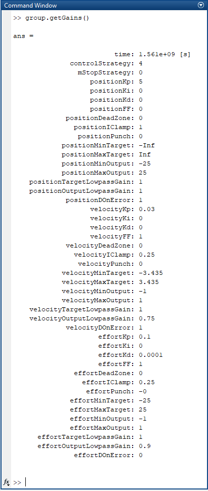
% Save gains to disk
gains = group.getGains();
HebiUtils.saveGains(gains, 'myGains.xml');

% Load gains from disk and send with guaranteed delivery
gains = HebiUtils.loadGains('myGains.xml');
HebiUtils.sendWithRetry(group, 'gains', gains);
Gains can be saved and loaded from disk using GroupInfo.write_gains and GroupCommand.read_gains.
# Saving gains from a group of modules:
group_info = group.request_info()

if group_info is not None:
  group_info.write_gains("myGains.xml")

# Loading gains from a file onto a group of modules:
group_cmd = hebi.GroupCommand(group.size)
group_cmd.read_gains("myGains.xml")
success = group.send_command_with_acknowledgement(group_cmd)
To save gains from or load gains onto a module, call the writeSafetyParameters and readSafetyParameters functions on the
hebi::GroupInfo and hebi::GroupCommand objects as follows:
// Saving gains from a group of modules:
GroupInfo group_info(group->size());
if (group->requestInfo(&group_info))
  group_info.writeGains("myGains.xml");

// Loading gains from a file onto a group of modules:
GroupCommand group_cmd(group->size());
group_cmd.readGains("myGains.xml");
bool success = group->sendCommandWithAcknowledgement(group_cmd);
Alternatively, individual gains can be accessed and set programmatically. The example below demonstrates programmatic doubling of the position P gain for each module in the group:
-
MATLAB
-
Python
-
C++
% Double position P gain
gains = group.getGains();
gains.positionKp = gains.positionKp * 2;
group.send('gains', gains);
You can see that there are associated gains fields within both the GroupCommand and GroupInfo classes.
# Double position P gain
group_info = hebi.GroupInfo(group.size)
group_command = hebi.GroupCommand(group.size)

# Reuse "group_info" as best practice
group_info = group.request_info(group_info)

group_command.position_kp = group_info.position_kp * 2.0

group.send_command(group_command)
Upon inspection of the C++ API class hierarchy, you will see that there are nested classes within both the hebi::Command and hebi::Info classes used to access individual gains:
// Double position P gain
hebi::GroupInfo group_info(group->size());
hebi::GroupCommand group_command(group->size());
group->requestInfo(&group_info);

for (int i = 0; i < group->size(); i++) {
    auto& info_kp =
        group_info[i].settings().actuator().positionGains().positionKp();
    auto& cmd_kp =
        group_command[i].settings().actuator().positionGains().positionKp();
    if (info_kp) {
        cmd_kp.set(info_kp.get() * 2.0);
    }
}
group->sendCommand(group_command);
For gain scheduling use cases with frequent gain changes, we recommend combining gain commands in the same Group "send" call as other commands to guarantee that everything arrives at the same time:
-
MATLAB
-
Python
-
C++
% Set gains
gains = GainStruct();
gains.positionKp = 5;

% Set desired targets
cmd = CommandStruct();
cmd.position = 0;

% Send at the same time
group.send(cmd, 'gains', gains);
group_command = hebi.GroupCommand(group.size)
# Set gains
group_command.position_kp = 5
# Set desired targets
group_command.position = 0
# Send at the same time
group.send_command(group_command)hebi::GroupCommand group_command(group->size());
// Set gains
for (int i = 0; i < group->size(); i++) {
group_command[i].settings().actuator().positionGains().positionKp().set(5);
}
// Set desired targets
group_command.setPosition(Eigen::VectorXd::Zero(group->size()));
// Send at the same time
group->sendCommand(group_command);Persisting Gains
Note that gains are not automatically persisted and get reset after reboot. The following code forces a persist such that the gains are maintained during a reboot. Note that persist should not be called in a loop due to significant overhead on the device.
-
MATLAB
-
Python
-
C++
% Send guaranteed and persist permanently (don't call this in a control loop)
HebiUtils.sendWithRetry(group, 'gains', gains, 'persist', true)
# Send with acknowledgement and persist permanently (don't call this in a control loop)
group_cmd.read_gains("myGains.xml")
group_cmd.save_current_settings = True
success = group.send_command_with_acknowledgement(group_cmd)// Send with acknowledgement and persist permanently (don't call this in a control loop)
group_cmd.readGains("myGains.xml");
for (int i = 0; i < group->size(); ++i)
group_cmd[i].saveCurrentSettings().set();
bool success = group->sendCommandWithAcknowledgement(group_cmd);Safety Parameters
The APIs can be used to read and modify the safety parameters (position and velocity limits, for example) on each device. As with gains, we recommend stored desired safety parmeters using the XML Safety Params Format and saving to/loading from disk with following the API functions:
-
MATLAB
-
Python
-
C++
The SafetyParamsStruct can be used to change the safety parameters.
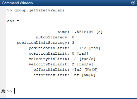
Safety parameters can be saved and loaded from disk using saveSafetyParams and loadSafetyParams.
% Save safety parameters to disk
safetyParams = group.getSafetyParams();
HebiUtils.saveSafetyParams(safetyParams, 'mySafetyParams.xml');

% Load safety params from disk and send with guaranteed delivery
safetyParams = HebiUtils.loadSafetyParams('mySafetyParams.xml');
HebiUtils.sendWithRetry(group, 'SafetyParams', safetyParams);
Safety parameters can be saved and loaded from disk using GroupInfo.write_safety_parameters and GroupCommand.read_safety_parameters.
# Saving safety parameter from a group of modules:
group_info = group.request_info()

if group_info is not None:
  group_info.write_safety_parameters("mySafetyParams.xml")

# Loading safety parameters from a file onto a group of modules:
group_cmd = hebi.GroupCommand(group.size)
group_cmd.read_safety_parameters("mySafetyParams.xml")
success = group.send_command_with_acknowledgement(group_cmd)
To save safety parameters from or load safety parameters onto a module, call the writeSafetyParameters and readSafetyParameters functions on the
hebi::GroupInfo and hebi::GroupCommand objects as follows:
// Saving safety parameters from a group of modules:
GroupInfo group_info(group->size());
if (group->requestInfo(&group_info))
  group_info.writeSafetyParameters("mySafetyParams.xml");

// Loading safety parameters from a file onto a group of modules:
GroupCommand group_cmd(group->size());
group_cmd.readSafetyParameters("mySafetyParams.xml");
bool success = group->sendCommandWithAcknowledgement(group_cmd);
Individual safety parameter values can also be accessed directly using the SafetyParamsStruct (MATLAB) or GroupCommand/GroupInfo objects (Python and C++):
-
MATLAB
-
Python
-
C++
% Limit position to +/- pi
safetyParams = group.getSafetyParams();
safetyParams.positionLimitStrategy = 3; % damped spring
safetyParams.positionMinLimit = -pi;
safetyParams.positionMaxLimit = +pi;
HebiUtils.sendWithRetry(group, 'SafetyParams', safetyParams);| For information regarding strategy values see SafetyParamsStruct. |
# Limit position to +/- pi
group_command = hebi.GroupCommand(group.size)
group_command.position_limit_min = -math.pi
group_command.position_limit_min = math.pi
group_command.min_position_limit_strategy = 'DampedSpring'
group_command.max_position_limit_strategy = 'DampedSpring'
group.send_command(group_command)
// Limit position to +/- pi
hebi::GroupCommand group_command(group->size());
for (int i = 0; i < group->size(); i++) {
group_command[i].settings().actuator().positionLimitMin.set(-M_PI);
group_command[i].settings().actuator().positionLimitMax.set(M_PI);
group_command[i].settings().actuator().minPositionLimitStrategy.set(PositionLimitStrategy::DampedSpring);
group_command[i].settings().actuator().maxPositionLimitStrategy.set(PositionLimitStrategy::DampedSpring);
}
group.sendCommand(group_command);Robot Model / Kinematics
We have created the Kinematics (MATLAB) / RobotModel (C++/Python) APIs to assist with computing forward and inverse kinematics, jacobians, and joint torques and forces. These APIs contain classes and functions to store and work with robot kinematic configurations.
Robot configurations can be loaded from XML files using the HEBI Robot Description Format (HRDF):
-
MATLAB
-
Python
-
C++
The loadHRDF method creates a HebiKinematics object:
% Loading a robot description (hrdf) from file
kin = HebiUtils.loadHRDF('hrdf/A-2580-06G.hrdf');
Each HebiKinematics object is a serial chain of bodies that describe the kinematic relation of a robot. The chain gets defined starting from the base of the device.
The hebi.robot_model module is used to load and work with robot kinematic configurations:
import hebi

# Load the RobotModel for a 6-DoF Arm
arm = hebi.robot_model.import_from_hrdf("hrdf/A-2580-06G.hrdf")
The hebi::RobotModel namespace is used to load and work with robot kinematic configurations:
// Load the RobotModel for a 6-DoF Arm
std::unique_ptr<hebi::robot_model::RobotModel> arm = hebi::robot_model::RobotModel::loadHRDF("hrdf/A-2580-06G.hrdf");
Make sure your HRDF file is saved at an appropriate location or loadHRDF will return an empty unique_ptr!
| Robot configurations can also be created programmatically using the MATLAB addBody MATLAB API, Python RobotModel functions, or C++ RobotModel functions. These methods and their named parameters correspond with kinematic types given in the Kinematic Body Types section as well as generic "rigid body" and "joint" types. However, it is strongly recommended that you use the define your kinematics in an HRDF file, and use the provided methods to load it into the API. |
Serial Chain Manipulators
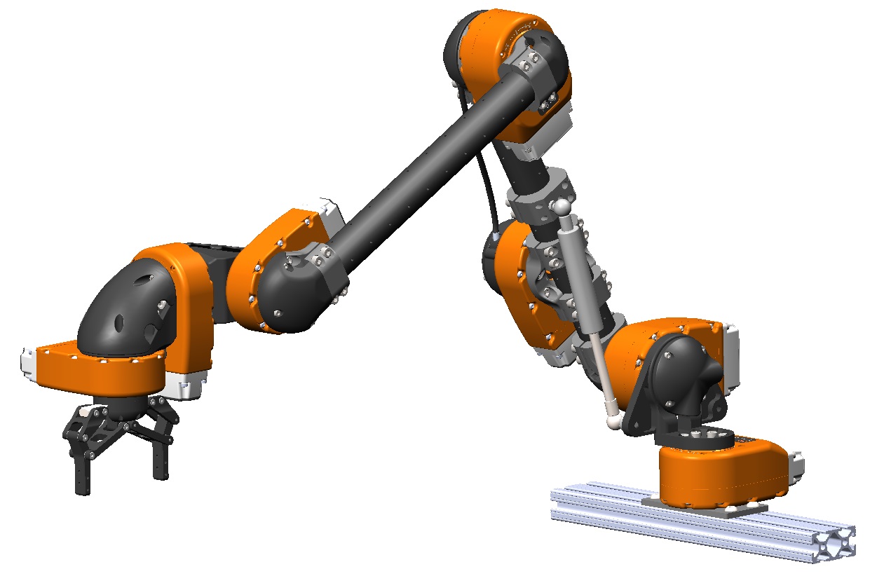
Many configurations are serial chains such as the 6-DoF T-Series Manipulator kit A-2580-06G:
<?xml version="1.0" encoding="UTF-8"?>
<!-- T-Series Arm (6-DoF with Gripper) -->
<robot version="1.6.0">
  <actuator type="T8-9"/>
  <bracket type="R8HeavyRightOutside"/>
  <actuator type="T8-16"/>
  <!-- Mass offset to account for mounted gripper actuator -->
  <link type="R8" extension="0.325" twist="pi" mass_offset="0.8"/>
  <actuator type="T8-9"/>
  <link type="R8" extension="0.325" twist="pi"/>
  <actuator type="T5-1"/>
  <bracket type="R8LightRight"/>
  <actuator type="T5-1"/>
  <bracket type="R8LightRight"/>
  <actuator type="T5-1"/>
  <end-effector type="R8Parallel"/>
</robot>
After loading into a HebiKinematics/RobotModel object using the "load HRDF" methods, the resulting object consists of a chain of elements that each represent either a rigid link or a dynamic joint element. The object starts at the baseFrame, and usually ends in an endEffector (but is not required to).
-
MATLAB
-
Python
-
C++
The firstJointFrame is the combination of the baseFrame and all static bodies up until the first joint. Details about an existing configuration can be accessed at runtime using getBodyInfo for general body information, and getJointInfo for joint specific information.
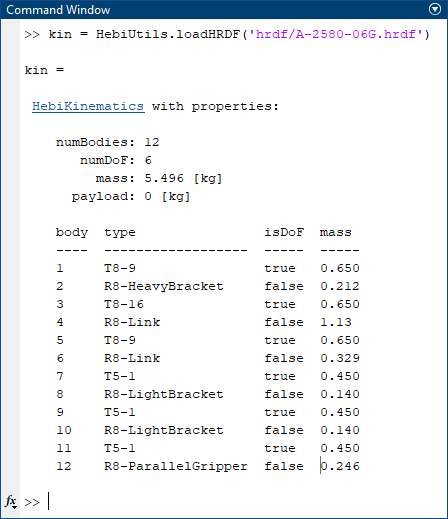
You can displaying the arm in an interactive Python shell:
>>> arm = hebi.robot_model.import_from_hrdf("hrdf/A-2580-06G.hrdf")
>>> arm
RobotModel with properties:

    body_count: 12
     dof_count: 6
          mass: 5.50 [kg]

    body  type             is_dof  mass [kg]
    ----  ---------------  ------  ---------
    0     T8-9             true       0.6500
    1     Bracket          false      0.2120
    2     T8-16            true       0.6500
    3     Link             false      1.1290
    4     T8-9             true       0.6500
    5     Link             false      0.3290
    6     T5-1             true       0.4500
    7     Bracket          false      0.1400
    8     T5-1             true       0.4500
    9     Bracket          false      0.1400
    10    T5-1             true       0.4500
    11    End Effector     false      0.2464
The base_frame, dof_count, get_frame_count, and element_count properties and methods provide high-level information about the RobotModel, and the https://files.hebi.us/docs/python/2.13.1/hebi/py_api.html#metadata functions contain more detailed information for each element of the RobotModel.
>>> print(arm.base_frame)
[[1. 0. 0. 0.]
 [0. 1. 0. 0.]
 [0. 0. 1. 0.]
 [0. 0. 0. 1.]]
>>> print(f"DOFs: {arm.dof_count}, Output frames: {arm.get_frame_count('output')}, Elements: {arm.element_count}")
DOFs: 6, Output frames: 12, Elements: 12
>>> arm.metadata[0]
Type:  Actuator
Model: T8-9
The base_frame, getDoFCount(), get_frame_count, and element_count properties and methods provide high-level information about the RobotModel, and the https://files.hebi.us/docs/python/2.13.1/hebi/py_api.html#metadata functions contain more detailed information for each element of the RobotModel.
std:cout << model->getBaseFrame() << "\n";
// 1 0 0 0
// 0 1 0 0
// 0 0 1 0
// 0 0 0 1

std::cout << "DOFs: " << model->getDoFCount() << ", Output frames: " << model->getFrameCount(hebi::robot_model::FrameType::Output) << "\n";
// DOFs: 6, Output frames: 12

std::vector<hebi::robot_model::MetadataBase> metadata;
model->getMetadata(metadata);
hebi::robot_model::ActuatorType actuator_type = metadata[0].asActuator()->actuatorType();
// actuator_type is hebi::robot_model::ActuatorType::T8_9
Multi-limbed Robots and Tree-Structures
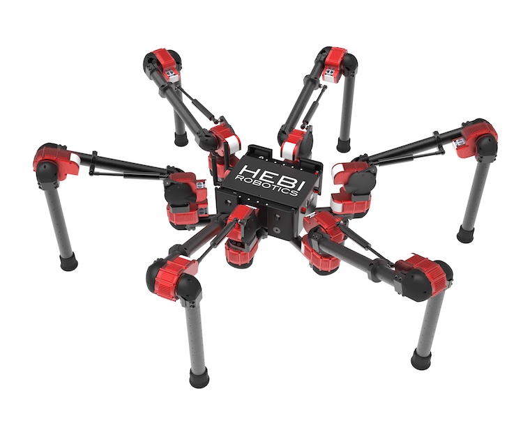
Some kits such as Daisy (A-2049-01) consist of multiple limbs that are attached to a shared chassis but effectively act independent of each other:
<?xml version="1.0" encoding="UTF-8"?>
<!--
    Leg Numbering / Chassis Coordinate convention:
    This should match ROS wheeled vehicle convention

    1 - - - 2           +x
        |                ^
    3 - - - 4            |
        |          +y <- o
    5 - - - 6             +z
-->
<robot version="1.3.0" description="Daisy">
    <rigid-body mass="0">
        <output rot="Rz(pi/6)"> <!-- leg 1 -->
            <rigid-body mass="0" output_trans="0.2375 0 0"/>
            <include path="daisyLeg-Left.hrdf"/>
        </output>
        <output rot="Rz(-pi/6)"> <!-- leg 2 -->
            <rigid-body mass="0" output_trans="0.2375 0 0"/>
            <include path="daisyLeg-Right.hrdf"/>
        </output>
        <output rot="Rz(pi/2)"> <!-- leg 3 -->
            <rigid-body mass="0" output_trans="0.1875 0 0"/>
            <include path="daisyLeg-Left.hrdf"/>
        </output>
        <output rot="Rz(-pi/2)"> <!-- leg 4 -->
            <rigid-body mass="0" output_trans="0.1875 0 0"/>
            <include path="daisyLeg-Right.hrdf"/>
        </output>
        <output rot="Rz(5*pi/6)"> <!-- leg 5 -->
            <rigid-body mass="0" output_trans="0.2375 0 0"/>
            <include path="daisyLeg-Left.hrdf"/>
        </output>
        <output rot="Rz(5*-pi/6)"> <!-- leg 6 -->
            <rigid-body mass="0" output_trans="0.2375 0 0"/>
            <include path="daisyLeg-Right.hrdf"/>
        </output>
        <output> <!-- chassis -->
            <include path="daisyChassis.hrdf"/>
            <end-effector/>
        </output>
    </rigid-body>
</robot>
Such tree structures defined in a single HRDF can be parsed using the APIs. The usage is slightly different depending on language to align with the capabilities and style of each:
-
MATLAB
-
Python
-
C++
The tree structure is loaded into a cell array of separate HebiKinematics objects representing each limb. Each one refers to the serial chain from the base frame to the desired endEffector indexed as they occur in the file.
% Loading a robot description (hrdf) from file
[~,~,limbs,jointIndices] = HebiUtils.loadHRDF('hrdf/Daisy.hrdf');
The additionally returned jointIndices list the actuator indices that are used in the chain. For example, Daisy consists of 18 actuators total, and leg 4 uses actuators 10-12.
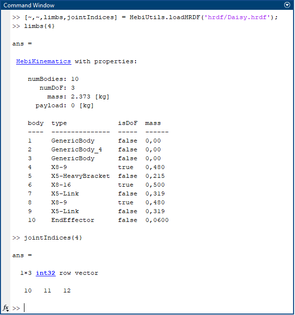
The RobotModel object directly represents the kinematic tree from the HRDF file, and frames are indexed in a depth-first ordering.
Using the RobotModel.get_sub_tree` function, you can create a RobotModel object that starts at a specified element.
This can be used to extract individual legs for the hexapod robot model, for example.
leg_1 = robot_model.get_subtree_with_root(element_idx=1)
Note that the base frame of this subtree is set to identity by default, and so to get locations of elements of this subtree relative to the parent RobotModel you need to either manually set the base frame or premultiply the kinematics by the input frame transform of the subtree root element within the parent RobotModel. Also note that a created subtree shares memory with the parent RobotModel, and should not be considered thread-safe from the parent.
|
The RobotModel object directly represents the kinematic tree from the HRDF file, and frames are indexed in a depth-first ordering.
Using the RobotModel::createSubtree` function, you can create a RobotModel object that starts at a specified element.
This can be used to extract individual legs for the hexapod robot model, for example.
std::unique_ptr<hebi::robot_model::RobotModel> leg_1 = robot_model.createSubtree(1);
Note that the base frame of this subtree is set to identity by default, and so to get locations of elements of this subtree relative to the parent RobotModel you need to either manually set the base frame or premultiply the kinematics by the input frame transform of the subtree root element within the parent RobotModel. Also note that a created subtree shares memory with the parent RobotModel, and should not be considered thread-safe from the parent.
|
Forward Kinematics
The APIs provide "forward kinematics" methods to compute the 4 x 4 homogeneous transform matrix for each element in the model, using specified values for the joint parameters. These transforms are returned as a vector of 4 x 4 matrices (or [4 x 4 x n] matrix in MATLAB), specified in the world frame. This world frame defaults to the input frame
of the base module, although a transformation can be prepended by setting the base frame of the HebiKinematics/RobotModel object.
Units of XYZ translation are in [m].
-
MATLAB
-
Python
-
C++
Use getForwardKinematics; transforms are returned as a [4 x 4 x numBodies] matrix.
% setup
% group = ...
% kin = ...

% loop
while true

    % read sensor values
    fbk = group.getNextFeedback();

    % calculate transforms from the world frame to the output frames of the individual bodies
    frames = kin.getForwardKinematics('OutputFrame', fbk.position);
    disp(frames(:,:,end)); % display end effector output

    % calculate transforms from the world frame to the centers of mass of the individual bodies
    CoM = kin.getForwardKinematics('CoMFrame', fbk.position);

    % calculate transform to only the end effector
    endEffectorFrame = kin.getForwardKinematicsEndEffector();

end
The get_forward_kinematics method computes the frames as a list of numpy 4 x 4 matrices. Use the frame_type argument to specify the desired frame type (see below). The length of the returned list depends on the selected frame type (which can be queried with get_frame_count):
group_feedback = hebi.GroupFeedback(group.size)
while True:
    # read sensor values
    if group.get_next_feedback(reuse_fbk=group_feedback) is None:
        continue

    # calculate transforms from the world frame to the output frames of the individual bodies
    output_frames = robot_model.get_forward_kinematics('output', group_feedback.position)

    # calculate transforms from the world frame to the centers of mass of the individual bodies
    com_frames = robot_model.get_forward_kinematics('com', group_feedback.position)

    # calculate transform to only the end effector(s)
    end_effector_frames = kin.get_forward_kinematics('end_effector', group_feedback.position)
It can be more efficient to reuse kinematics matrices when operating in a loop:
group_feedback = hebi.GroupFeedback(group.size)
output_frames = [np.ndarray(shape=(4,4), dtype=np.float64)] * robot_model.get_frame_count('output')
while True:
    # read sensor values
    if group.get_next_feedback(reuse_fbk=group_feedback) is None:
        continue
    # calculate transforms from the world frame to the output frames of the individual bodies
    robot_model.get_forward_kinematics('output', group_feedback.position, output_frames)
The RobotModel.get_end_effector
method is a shortcut for just obtaining the output transform of the last frame
in the RobotModel object; for a RobotModel with multiple end effectors this will return the first.
transform = model.get_end_effector(angles)
print(f"4x4 transform from base to end effector: {transform}")
Use the RobotModel getForwardKinematics function (aliased as RobotModel::getFK); transforms are returned as a list of Eigen::Matrix4d matrices. Use the hebi::FrameType argument to specify the desired frame type (see below). The length of the returned list depends on the selected frame type (which can be queried with getFrameCount):
A hebi::robot_model::Matrix4dVector object is passed in to the getFK function, and is resized as necessary and filled in with the computed transforms (in order of the bodies in the RobotModel object). This type is simply a std::vector containing Eigen::Matrix4d elements; due to memory alignment considerations Eigen types in std containers must use particular allocators for certain C++ versions and compilers, and so we provide this convenience typedef. (See https://eigen.tuxfamily.org/dox-devel/group__TopicStlContainers.html for more information on this requirement)
hebi::GroupFeedback feedback(group->size);
// Best not to reallocate each time through the loop
hebi::robot_model::Matrix4dVector frames_out;
hebi::robot_model::Matrix4dVector frames_com;
hebi::robot_model::Matrix4dVector frames_ee;
while (true) {
  // read sensor values
  if (!group->getNextFeedback(&feedback))
    continue;
  // calculate transforms from the world frame to the output frames of the individual bodies
  robot_model->getForwardKinematics(hebi::robot_model::FrameType::Output, feedback.getPosition(), frames_out);

  // calculate transforms from the world frame to the centers of mass of the individual bodies; use aliased `getFK` here
  robot_model->getFK(hebi::robot_model::FrameType::CenterOfMass, feedback.getPosition(), frames_com);

  // calculate transform to only the end effector(s)
  robot_model->getForwardKinematics(hebi::robot_model::FrameType::EndEffector, feedback.getPosition(), frames_ee);
}
The RobotModel::getEndEffector method is a shortcut for just obtaining the output transform of the last frame in the RobotModel object; for a RobotModel with multiple end effectors this will return the first.
// Set up hebi::RobotModel object "model" and Eigen::VectorXd "angles" as above...
...
Eigen::Matrix4d transform;
model.getEndEffector(angles, transform);
std::cout << "4x4 transform from base to end effector: " << std::endl
          << transforms[i] << std::endl;
Full API documentation of these functions is available here.
There are several types of frames available:
-
Each element in the RobotModel (corresponding to an element in the HRDF file) has an "input" frame (see note below).
-
Each non-"end effector" element in the RobotModel has one or more "output" frames (usually a single output frame, although rigid-body or specific bracket elements may have multiple outputs to form a tree).
-
Each "end effector" element has an 'end_effector' frame; for kinematic chains this is typically a single element, but for kinematic trees this could be larger (e.g., 6 for a hexapod, one per foot).
-
Each non-"joint" element has a "center of mass" frame. Note that an "Actuator" has a center of mass, as the "joint" robot model element represents a pure massless joint.
-
Some elements may have an associated "mesh" frame, which indicates the transform to its 3D geometry mesh used for visualization.
-
There is an additional "payload" frame for each end effector; see the payload section below.
API differences:
There are a couple slight differences between the APIs regarding the kinematic frames:
-
As MATLAB’s kinematic object only represents pure kinematic chains, the "input" frames would just be the HebiKinematics' base frame and all of the output frames except the final one. Therefore, there is not a corresponding "InputFrame" frame type in MATLAB.
-
Pure joints in MATLAB are still returned in the "center of mass" frames.
-
There is no "mesh" frame type in MATLAB.
-
In MATLAB, the "payload" frames are read with separate calls to the
getPayloadfunctions.
Jacobians
We can also use the HebiKinematics/RobotModel object to obtain the Jacobian, or the partial derivatives of the forward kinematics equation.
This relates the joint velocities to the linear and angular velocity of each body in the system.
The HebiKinematics/RobotModel objects have "get jacobian" methods to calculate this for given joint angles using the same "frame type" and "position" parameters as for forward kinematics calls shown above.
The Jacobian in returned as a set of matrices, one for each body in the RobotModel object.
Each matrix is of size 6 x numDoF.
Rows 1 - 3 of this matrix corresponds to this body’s linear velocities [m/s] along the X-Y-Z axes in the world frame, while rows 4 - 6 correspond to rotational velocities [rad/s] about the X-Y-Z axes in the world frame.
The columns define the contributions to these linear and rotational velocities that would be a result of the respective degree of freedom instantaneously moving at unit velocity (e.g., a rotational joint being driven at 1 rad/s).
-
MATLAB
-
Python
-
C++
The getJacobian method calculates and returns the Jacobian as a single [6 x numDof x numBodies] matrix:
% Jacobian for all body outputs
J = kin.getJacobian('OutputFrame', fbk.position);

% Jacobian for all body centers of mass
J = kin.getJacobian('CoMFrame', fbk.position);

% Jacobian for only the end effector output frame
J = kin.getJacobianEndEffector();
As with the forward kinematics, we provide versions for the (first) end effector
(which just returns a single 6 x numDoF matrix) as well as the entire system.
# Set up hebi.robot_model.RobotModel object "model" and np.ndarray "angles" as above...
...

# Get Jacobian for all bodies:
transforms = model.get_jacobians('output', angles)

# Get Jacobian for center of mass frames (useful for computing gravity or dynamics compensation torques):
transforms = model.get_jacobians('com', angles)

# Get Jacobian for (first) end effector:
# 'reuse_jacobians' is an optional argument, but using it to provide
# a previously computed jacobians list amortizes the time to call this function
transform = model.get_jacobian_end_effector(angles, reuse_jacobians=transforms)
Full API documentation of these functions is available here.
As with the forward kinematics, we provide versions for the (first) end effector
(which just returns a single 6 x numDoF matrix) as well as the entire system.
Note that the matrices are now of type Eigen::MatrixXd and MatrixXdVector.
// Set up hebi::RobotModel object "model" and Eigen::VectorXd "angles" as above...
...

// Get Jacobian for all bodies:
MatrixXdVector transforms;
model.getJ(hebi::robot_model::FrameType::Output, angles, transforms);

// Get Jacobian for center of mass frames (useful for computing gravity or dynamics compensation torques):
model.getJ(hebi::robot_model::FrameType::CenterOfMass, angles, transforms);

// Get Jacobian for (first) end effector:
Eigen::MatrixXd transform;
kin.getJEndEffector(angles, transform);
Full API documentation of these functions is available here.
Inverse Kinematics
The RobotModel object also provides a method for computing joint angles that solve the inverse kinematics, according to a number of objectives and constraints. In other words, these methods help to find the joint angles to move specified parts of your robot to desired locations in the world.
Note that the implementation of this function relies on a local optimization, and so is highly dependent on the initial joint angles that are provided as the seed for the search.
-
MATLAB
-
Python
-
C++
The getInverseKinematics method computes the joint positions associated to a desired end-effector configuration. The end effector is assumed to be the last body in the kinematic chain.
There are a variety of optimization criteria that can be combined depending on the application. Available parameters include:
| Parameter | End Effector Target | Comments |
|---|---|---|
|
xyz position (m) |
|
|
z-axis orientation of end effector |
|
|
3-DoF orientation of end effector |
|
|
Initial seed for the numerical optimization. This is an important parameter for IK to work well. See the IK section of Core Concepts for more details. Defaults to all zeros. |
|
|
Maximum allowed iterations of the numerical optimization before returning. |
% Inverse kinematics on carthesian coordinates
xyz = [0 0 0];
waypoints = kin.getInverseKinematics('xyz', xyz);

% Inverse kinematics for full 6 dof
xyz = [0 0 0];
so3 = eye(3);
positions = kin.getIK('xyz', xyz, 'so3', so3);
The desired objectives and constraints should be passed to the RobotModel.solve_inverse_kinematics function as a series of arguments - any number are permitted, but there are limitations in which can be used together.
As an example, the solve_inverse_kinematics function is used to find joint angles that move the end effector to a given position (but other objectives can be used to solve the IK problem for other frames):
# Set up RobotModel object "model" and vector "angles" as above...
...

target_xyz = [0.4, 0.0, 0.2]
initial_joint_angles = np.array(model.dof_count)

# Fill in 'initial joint angles', perhaps with feedback from the robot.
...

end_effector_position_objective = hebi.robot_model.endeffector_position_objective(target_xyz)

################################################################################
# Demonstration of using a single objective:
################################################################################

ik_result_joint_angles = model.solve_inverse_kinematics(initial_joint_angles,
  end_effector_position_objective)

################################################################################
# Demonstration of using a custom objective:
################################################################################

def custom_objective_func(positions, errors, user_data):
  # This objective prefers joint angles that sum to '2'
  errors[0] = 2.0 - positions.sum()

user_data = None # can be anything

custom_objective = hebi.robot_model.custom_objective(1, custom_objective_func, user_data)

ik_result_joint_angles = model.solve_inverse_kinematics(initial_joint_angles,
  custom_objective)

################################################################################
# Demonstration of using a multiple objectives:
################################################################################

# Set joint limit constraints:
min_positions = [-math.pi, -1.0, -1.0]
max_positions = [math.pi, 1.0, 1.0]

joint_limit_constraint = hebi.robot_model.joint_limit_constraint(min_positions,
  max_positions)

ik_result_joint_angles = model.solve_inverse_kinematics(initial_joint_angles,
  end_effector_position_objective,
  joint_limit_constraint)
Full API documentation of these functions is available here.
The desired objectives and constraints should be passed to the solveIK function as a series of arguments; any number are permitted, but there are limitations in which can be used together. In future API releases, the IKResult return structure will contain more information about the optimization result.
Here is an example of using the solveIK function to find joint angles that move the end effector to a given position (but other objectives can be used to solve the IK problem for other frames):
// Set up hebi::RobotModel object "model" and Eigen::VectorXd "angles" as above...
...

Eigen::Vector3d target_xyz;
target_xyz << 0.4, 0.0, 0.2;
Eigen::VectorXd initial_joint_angles(model->getDoFCount());
Eigen::VectorXd ik_result_joint_angles(model->getDoFCount());

// Fill in 'initial joint angles', perhaps with feedback from the robot.
...

////////////////////////////////////////////////////////////////////////////
// Demonstration of using a single objective:
////////////////////////////////////////////////////////////////////////////

model.solveIK(
  initial_joint_angles,
  ik_result_joint_angles,
  kinematics::EndEffectorPositionObjective(target_xyz)
);

////////////////////////////////////////////////////////////////////////////
// Demonstration of using a custom objective:
////////////////////////////////////////////////////////////////////////////

model.solveIK(
  initial_joint_angles,
  ik_result_joint_angles,
  robot_model::CustomObjective<1>(
    [](const std::vector<double> positions, std::array<double, 1>& errors)
    {
      // Add up all the joint angles
      double sum = 0;
      for (auto p : positions)
        sum += p;
      // This objective prefers joint angles that sum to '2'
      errors[0] = 2 - sum;
    }
  )
);

////////////////////////////////////////////////////////////////////////////
// Demonstration of using multiple objectives (allowed through variadic templates)
////////////////////////////////////////////////////////////////////////////

// Set joint limit constraints:
Eigen::VectorXd min_positions(model->getDoFCount());
min_positions << -M_PI, -1.0f, -1.0f;
Eigen::VectorXd max_positions(model->getDoFCount());
max_positions << M_PI, 1.0f, 1.0f;

model.solveIK(
  initial_joint_angles,
  ik_result_joint_angles,
  kinematics::EndEffectorPositionObjective(target_xyz),
  kinematics::JointLimitConstraint(min_positions, max_positions)
);
Full API documentation of these functions is available here.
Computing Compensatory Torques
Modeling required torques appropriately can significantly improve tracking while also improving stability. Please take a look at the Motion Control tutorial for an in-depth explanation with visual examples. The APIs provide methods for computing gravity and dynamics compensation torques, as shown in the following sections.
Gravity Compensation
Calculating the joint torques required to counteract the force of gravity on a robot arm can be done using the transpose of the Jacobian matrix.
Applying these torques as feed forward values reduce the necessary contribution from the position PID loop, allowing improved tracking performance with lower and more stable PID gains. The HebiKinematics/RobotModel classes provide methods to compute these gravity compensation forques and forces.
| The Arm API, described later in the documentation, provides this functionality automatically as a default plugin. |
-
MATLAB
-
Python
-
C++
Use the getGravCompEfforts method as follows:
% Compensate gravity at current position
fbk = group.getNextFeedback();
gravityVec = [0 0 -1]; % Direction of gravity. Does not need to be normalized.
efforts = kin.getGravCompEfforts(fbk.position, gravityVec);
Use the RobotModel.get_grav_comp_efforts method as follows:
# Compensate gravity at current position
feedback = group.get_next_feedback;
# Direction and magnitude of gravity
gravity = np.array([0, 0, -9.81])
efforts = robot_model.get_grav_comp_efforts(feedback.position, gravity)
Use the RobotModel getGravCompEfforts method as follows:
// This is resized as necessary by the "getGravCompEfforts" function
Eigen::VectorXd efforts;

// Direction and magnitude of gravity, relative to the base of your robot model:
Eigen::Vector3d gravity(0, 0, -9.81);
robot_model->getGravCompEfforts(feedback.getPosition(), gravity, efforts);
If you are not sure where gravity is coming from, an easy way to figure out the direction of gravity is to look at the orientation values of a device. The orientation quaternion is determined by locally fusing the accelerometers and gyroscopes and may be used while the robot is moving.
-
MATLAB
-
Python
-
C++
% automatically determine direction of gravity based on the local pose filter of the first joint:
fbk = group.getNextFeedbackFull();
q = [ fbk.orientationW(1), ...
      fbk.orientationX(1), ...
      fbk.orientationY(1), ...
      fbk.orientationZ(1) ];
baseRotMat = HebiUtils.quat2rotMat(q);
gravityVec = -baseRotMat(3, 1:3)';

% dealing with non identity base frames
imuFrame = kin.getFirstJointFrame();
gravityVec = imuFrame(1:3,1:3)' * gravityVec;
# automatically determine direction of gravity based on the local pose filter of the first joint
fbk = group.get_next_feedback()
# could use quat -> rotation matrix function from other libraries as well here
gravity = hebi.arm._gravity_from_quaternion(fbk.orientation[0]) * 9.81Note if the orientation feedback is not coming from a module that isn’t the base frame, you will need to premultiply the gravity vector by the input frame of that module
#include "util/grav_comp.hpp" // in hebi-cpp API sources; for gravityfromQuaternion function

// automatically determine direction of gravity based on the local pose filter of the first joint
group->getNextFeedback(feedback);
hebi::Quaternionf orientation = feedback[0].imu().orientation().get();
// could use quat -> rotation matrix function from other libraries as well here
gravity = hebi::util::gravityFromQuaternion(orientation) * 9.81;
Note if the orientation feedback is not coming from a module that isn’t the base frame, you will need to premultiply the gravity vector by the input frame of that module
The following example commands a "weightless" gravity-compensated mode that allows users to touch a robot arm and move it around freely in space. This is often useful control mode for an operator to teach waypoints for teach-repeat applications.
-
MATLAB
-
Python
-
C++
% Keep the robot in a weight-free teach mode
cmd = CommandStruct();
while true
    fbk = group.getNextFeedback();
    cmd.effort = kin.getGravCompEfforts(fbk.position, gravityVec);
    group.send(cmd);
end
# Compensate gravity at current position
feedback = group.get_next_feedback;
# Direction and magnitude of gravity, relative to the base of your robot model
gravity = np.array([0, 0, -9.81])
# Pre-allocate returned vector and command/feedback so these does not happen
# continually in loop
efforts = np.zeros(robot_model.size)
feedback = hebi.GroupFeedback(group.size)
command = hebi.GroupCommand(group.size)
while not stop_loop:
if group.get_next_feedback(reuse_fbk=feedback) is None:
continue
robot_model.get_grav_comp_efforts(feedback.position, gravity, output=efforts)
command.effort = efforts
group.send_command(command)hebi::GroupFeedback feedback(group->size());
hebi::GroupCommand command(group->size());
// This is resized as necessary by the "getGravCompEfforts" function
Eigen::VectorXd efforts;
// Direction and magnitude of gravity, relative to the base of your robot model:
Eigen::Vector3d gravity(0, 0, -9.81);
while (!stop_loop) {
if (!group->getNextFeedback(feedback))
continue;
robot_model->getGravCompEfforts(feedback.getPosition(), gravity, efforts);
command.setEffort(effort);
group->sendCommand(command);
}Dynamics Compensation
The "dynamics comp efforts" methods compute the torques (or forces) that are required to accelerate the body masses as determined from the specified positions, velocities, and accelerations. Typically the target positions, velocities, and accelerations are generated from following a smooth trajectory (as described in the trajectories section below), and refer to the commanded values along this trajectory, while the feedback position is also passed into the function and used (as with the gravity compensation function) to generate the Jacobian at the current configuration.
-
MATLAB
-
Python
-
C++
The getDynamicCompEfforts function is used to calculate the required torques:
% Calculate required efforts to compensate for desired accelerations
efforts = kin.getDynamicCompEfforts(...
    fbk.position, ...
    cmdPositions, ...
    cmdVelocities, ...
    cmdAccelerations);
# Calculate required efforts to compensate for desired accelerations
robot_model.get_dynamics_comp_efforts(fbk.position, cmd_position, cmd_velocity, cmd_acceleration)// Calculate required efforts to compensate for desired accelerations
robot_model.getDynamicsCompEfforts(fbk.getPosition(), cmd_position, cmd_velocity, cmd_acceleration);Adjusting Payload
Each end effector in the HebiKinematics/RobotModel object can have an associated "payload" point pass at a specified translation from the input of the end effector. The get and set payload methods provide a way to dynamically specify this payload. The payload gets used for calculating efforts to compensate for gravitational effects and joint accelerations, but currently has no effect on any other functionality.
-
MATLAB
-
Python
-
C++
The setPayload method allows the mass and center of mass for the payload to be set:
% Pick up an object with the specified mass and CoM (xyz distance from the end effector output frame)
mass = 1; % [kg]
com = [0.1 0 0]; % xyz distance in [m]
kin.setPayload(mass, 'CoM', com);

% Remove payload
kin.setPayload(0);
The RobotModel.set_payload function allows the mass and center of mass for the payload to be set:
# Pick up an object with the specified mass and CoM (xyz distance from the end effector output frame)
mass = 1 # [kg]
com = np.array([0.1 0 0]) #xyz distance in [m]
robot_model.set_payload(mass=mass, com=com)

# Remove payload
robot_model.set_payload(mass=0)
If there are multiple end effectors, you can select which to set the payload on using the index argument:
# Set payload of the 3rd end effector
robot_model.set_payload(index=2, mass=mass, com=com)
The payload can be retrieved with the RobotModel.get_payload function:
com = np.array([0 0 0])
mass = robot_model.get_payload(index=0, com_out=com)
The RobotModel setPayload and setPayloadCenterOfMass functions allows the mass and center of mass for the payload to be set:
// Pick up an object with the specified mass and CoM (xyz distance from the end effector output frame)
double mass = 1; // [kg]
Eigen::Vector3d com{0.1, 0, 0}; // xyz distance in [m]
size_t end_effector_index = 0;

robot_model->setPayload(end_effector_index, mass);
robot_model->setPayloadCenterOfMass(end_effector_index, com)

// Remove payload
robot_model->setPayload(end_effector_index, 0);
If there are multiple end effectors, you can select which to set the payload on using the end_effector_index argument, or set values on all simultaneously:
// Set payload of 3 end effectors
Eigen::VectorXd masses(3);
masses << 0.1, 0.5, 0.1;
robot_model->setPayloads(masses);
The payload can be retrieved with the getPayload and getPayloadCenterOfMass functions:
double mass = robot_model->getPayload(end_effector_index);
Eigen::Vector3d com = robot_model->getPayloadCenterOfMass(end_effector_index);
Trajectories
A trajectory is a (smooth) motion through two or more waypoints (specific joint position for each module in the robot).
A trajectory defines the position, velocity, and acceleration for each module at each point in time, from the start to end of the trajectory.
We provide trajectory generation APIs to create smooth trajectories through waypoints with specifiable velocity and acceleration constraints.
The generated trajectories have the property that they smoothly accelerate and decelerate with "minimum jerk" and are similar to human movement.
Please check the Trajectories tutorial for more information.
| For the common case of a fixed-base manipulator, the logic for creating and executing trajectories is wrapped within the Arm API, and so you do not need to call these functions directly. However, it is still useful to have a basic understanding of the trajectories being executed when using the Arm API. |
| More traditional robot arms usually are controlled by defining waypoints and some motion parameters (e.g., maximum acceleration), as opposed to the joint-level control our API provides at the lowest level. The trajectory API provides a way to define motions in a similar high-level way as these traditional systems, while still allowing access to control and feedback at a lower level. |
Creating Trajectories
Joint trajectories are created by defining waypoints (position, velocity, and acceleration) for the trajectory to pass through at specified times.
The API functions to create a trajectory take these times and waypoints, and compute minimum jerk trajectories that can be sampled.
Unspecified velocity and acceleration constraints default to zero start and end conditions with unconstrained waypoints in between.
The following code creates a sample trajectory between 6 position waypoints for a single actuator, using the unconstrained quadratic programming solver:
-
MATLAB
-
Python
-
C++
First create a HebiTrajectoryGenerator object, and then call the newJointMove method. on it.
% Setup
trajGen = HebiTrajectoryGenerator();

% Note that you will usually want a trajectory to start at your robot's current commanded joint position
current_position = 0

% Create trajectory
positions = [current_position pi 3 2.5 1 0];
time = [0 1 2 3 4 5];
trajectory = trajGen.newJointMove(positions, 'time', time);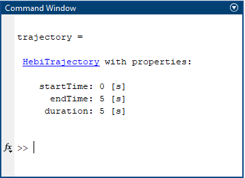
The Trajectory class is used to generate and access trajectory motions.
import hebi
import numpy as np
import math

# Populate variable 'current_position' with position feedback
current_position = 0

# Each column is a separate waypoint.
# Each row is a different joint.
num_joints = 1
pos = np.empty((num_joints, 6))

# Would normally have a set of positions for each joint
pos[0,:] = np.array([current_position, math.pi, 3, 2.5, 1, 0])

# The times to reach each waypoint (in seconds)
time = np.array([0, 1, 2, 3, 4, 5])

# Define trajectory (could also pass in velocity, and acceleration waypoint constraints)
trajectory = hebi.trajectory.create_trajectory(time, pos)
The hebi::trajectory::Trajectory class is used to generate and access trajectory motions.
// Position, velocity, and acceleration waypoints.  Each column is a separate
// waypoint; each row is a different joint.
const int num_joints = 1;
Eigen::MatrixXd positions(num_joints,5);
positions << current_position[0], M_PI, 3, 2.5, 1, 0;
// For multiple joints, you would do something like:
// positions << current_position[0], 1, 2, 3,
//              current_position[1], 2, 1, 0;

// The times to reach each waypoint (in seconds)
Eigen::VectorXd time(6);
time << 0, 1, 2, 3, 4, 5;

// Define trajectory (could also pass in velocity, and acceleration waypoint constraints)
auto trajectory = hebi::trajectory::Trajectory::createUnconstrainedQp(time, positions);
The trajectory can be evaluated at a specified time using tbe "get state" function. Note that times outside the duration of the trajectory will clip to the start/end of the trajectory rather than extrapolate.
-
MATLAB
-
Python
-
C++
Use getState to evaluate the trajectory.
% Evaluate state at specified time (scalar or vector)
[pos, vel, accel] = trajectory.getState(2);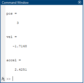
t = 2.0
pos_cmd, vel_cmd, accel_cmd = trajectory.get_state(t)
Eigen::VectorXd pos_cmd(num_joints);
Eigen::VectorXd vel_cmd(num_joints);
double t = 2.0;
// Pass "nullptr" in to ignore a returned value.
trajectory->getState(t, &pos_cmd, &vel_cmd, nullptr);Executing Trajectories
Trajectories are designed to be executed/evaluated in a non-blocking manner so that users can dynamically react to changes in the environment such as hitting unforeseen obstacles or when following a moving target. To play through the trajectory object, we query the position, velocity, and acceleration at each point in time, and send appropriate commands to the robot. Note that acceleration can not be (meaningfully) directly sent to the actuator, but with knowledge of the dynamics this can be converted to a torque or force to compensate for this acceleration. For improved control, we recommend adding effort commands that are the summation of torques/forces that compensate for gravity and torques/forces that compensate for this acceleration (see Compensatory Torques).
-
MATLAB
-
Python
-
C++
% Setup single joint
group = HebiLookup.newGroupFromNames('*', 'X-001');
kin = HebiKinematics();
kin.addBody('X5-1');
trajGen = HebiTrajectoryGenerator(kin);
trajGen.setAlgorithm('UnconstrainedQp'); % MinJerk trajectories
trajGen.setSpeedFactor(0.5); % Slow down to half of max speed

% Create trajectory through multiple waypoints
nWaypoints = 5;
positions = rand(nWaypoints, kin.getNumDoF());
trajectory = trajGen.newJointMove(positions);

% Execute trajectory in position and velocity
cmd = CommandStruct();
t0 = tic();
t = toc(t0);
while t < traj.getDuration()
    t = toc(t0);

    % React to something (e.g. position error or effort threshold)
    fbk = group.getNextFeedback();
    if fbk.position - fbk.positionCmd > 0.1
        group.send(CommandStruct()); % turn off commands
        error('Reacting to something...');
    end

    % Get target state at current point in time
    [pos, vel, accel] = traj.getState(t);

    % Command position/velocity
    cmd.position = pos;
    cmd.velocity = vel;
    group.send(cmd);

end| In MATLAB, HebiTrajectoryGenerator.executeTrajectory is a utility method provided to assist with simple movements in a blocking manner. However, this functionality is considered deprecated and we recommend using HebiArm instead. |
import hebi
import time

# Follow the trajectory
cmd = hebi.GroupCommand(num_joints)

pos_cmd = np.array(num_joints, dtype=np.float64)
vel_cmd = np.array(num_joints, dtype=np.float64)

duration = trajectory.duration
t0 = time.time()
t = 0
while (t < duration):
  t = time.time() - t0
  pos_cmd, vel_cmd, _ = trajectory.get_state(t)
  cmd.position = pos_cmd
  cmd.velocity = vel_cmd
  group.send_command(cmd)

  # Serves to rate-limit the loop:
  group.get_next_feedback()
// Helper function to get current time in seconds, starting
// from the first call to this function
auto getTime = []() {
using clock = std::chrono::steady_clock;
static const clock::time_point start_time = clock::now();
return (std::chrono::duration<double>(clock::now() - start_time)).count();
}
// Follow the trajectory
hebi::GroupCommand cmd(num_joints);
hebi::GroupCommand fbk(num_joints);
Eigen::VectorXd pos_cmd(num_joints);
Eigen::VectorXd vel_cmd(num_joints);
double duration = trajectory->getDuration();
double t = 0;
while (t < duration) {
double t = getTime();
// Pass "nullptr" in to ignore a term.
trajectory->getState(t, &pos_cmd, &vel_cmd, nullptr);
cmd.setPosition(pos_cmd);
cmd.setVelocity(vel_cmd);
group->sendCommand(cmd);
// Serves to rate-limit the loop:
group->getNextFeedback(fbk);
}Visualizing Trajectories
-
MATLAB
-
Python
-
C++
The MATLAB API provides a method to visualize a trajectory directly:
You can visualize the trajectory using the provided HebiUtils.plotTrajectory utility
% Visualize trajectory
HebiUtils.plotTrajectory(trajectory);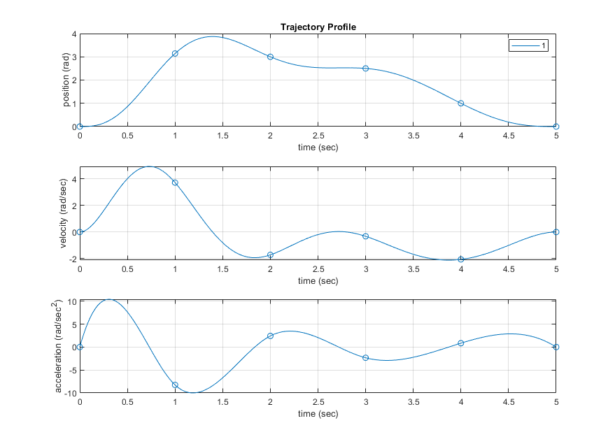
No direct "plot_trajectory" method available.
No direct "plotTrajectory" method available.
Alternatively, you can sample the trajectory at a given frequency and create a custom visualization:
-
MATLAB
-
Python
-
C++
% Visualize trajectory
figure(); hold on; grid on;

% Position / Velocity / Acceleration profile
t = 0:0.01:trajectory.getDuration();
[pos, vel, accel] = trajectory.getState(t);
plot(t, pos);
plot(t, vel);
plot(t, accel);

% Superimpose target position waypoints
tWaypoint = trajectory.getWaypointTime();
plot(tWaypoint, trajectory.getState(tWaypoint), 'bo');

% Axes labels
title('Joint Trajectory');
ylabel('Value [rad, rad/s, rad/s^2]');
xlabel('Time [s]');
legend Position Velocity Acceleration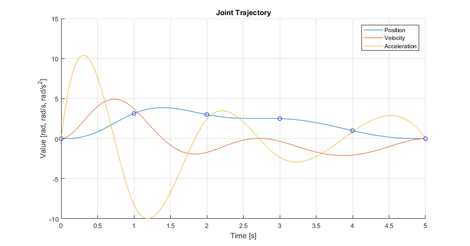
Here we use the hebi_charts plotting library. This library is available as an independent download, and is currently in beta, but you can download the latest version from here:
import hebi_charts
import hebi
import numpy as np
import math

def main():
    # Make trajectory:
    wp_pos = np.empty((1, 6), dtype=np.float64)
    wp_pos[0,:] = np.array([0, math.pi, 3, 2.5, 1, 0], dtype=np.float64)
    wp_t = np.array([0, 1, 2, 3, 4, 5], dtype=np.float64)
    trajectory = hebi.trajectory.create_trajectory(wp_t, wp_pos)

    # Set up charts
    window = hebi_charts.GridWindow.create()
    window.show()
    chart = window.add_line_chart()
    chart.set_title("Joint Trajectory")
    chart.get_axis_x().set_name("Time")
    chart.get_axis_x().set_unit("s")
    chart.get_axis_y().set_name("Value")
    chart.get_axis_y().set_unit("rad, rad/s, rad/s^2")
    pos_line = chart.add_line("Position")
    vel_line = chart.add_line("Velocity")
    acc_line = chart.add_line("Acceleration")

    # Sample trajectory and plot
    t = 0
    resolution = 0.01
    duration = trajectory.duration
    while t < duration:
        p, v, a = trajectory.get_state(t)
        pos_line.add_point(t, p)
        vel_line.add_point(t, v)
        acc_line.add_point(t, a)
        t += resolution

    window.wait_until_closed()

# Due to interaction on some OSes GUI libraries, must pass main function to the "runApplication" call
hebi_charts.runApplication(main)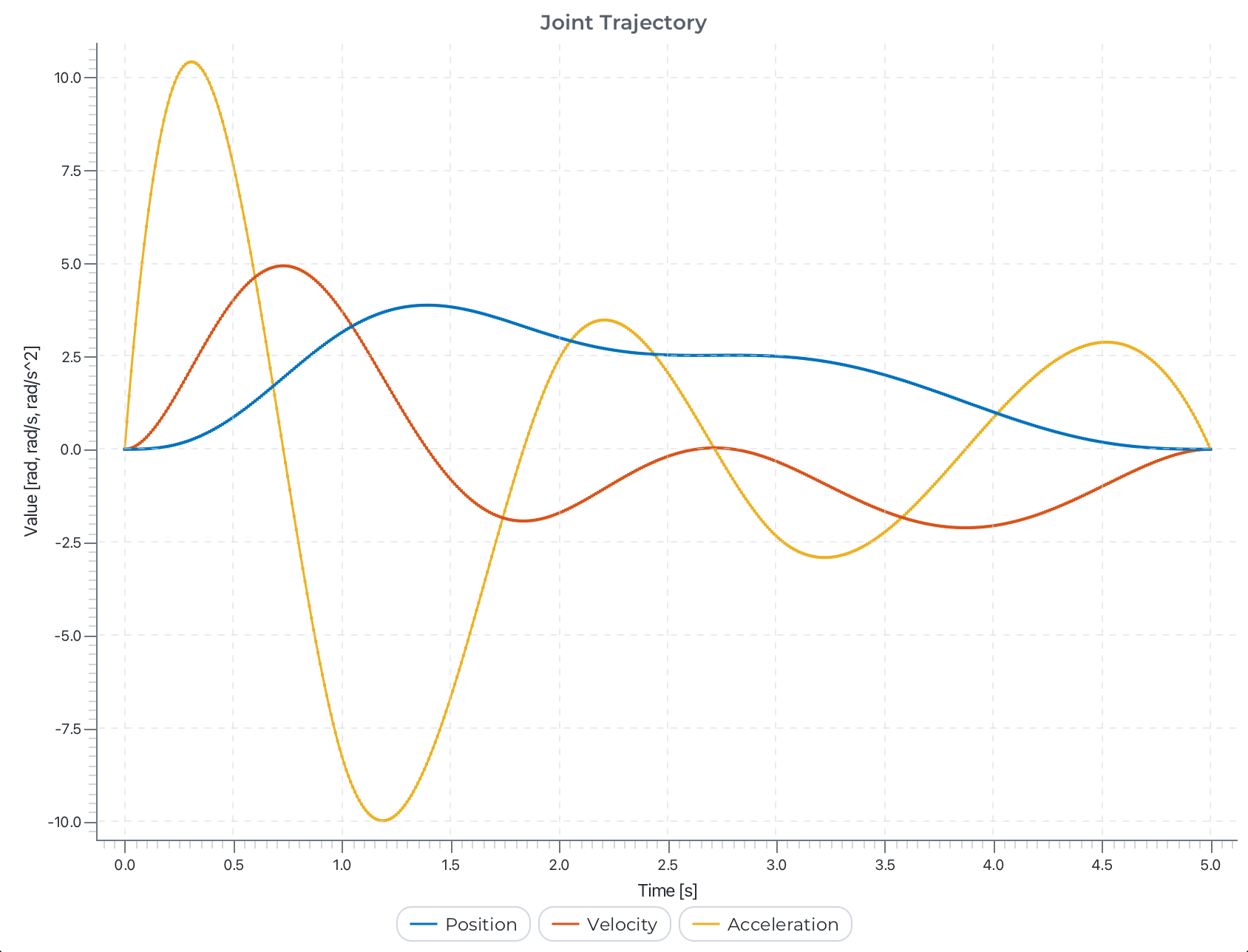
Here we use the hebi_charts plotting library. This library is available as an independent download, and is currently in beta, but you can download the latest version from here:
#include "hebi_charts.hpp"
#include "trajectory.hpp"

int plot(int argc, char** argv) {
  // Make trajectory:
  Eigen::MatrixXd wp_positions(1, 6);
  wp_positions << 0, M_PI, 3, 2.5, 1, 0;
  Eigen::VectorXd wp_time(6);
  wp_time << 0, 1, 2, 3, 4, 5;
  auto trajectory = hebi::trajectory::Trajectory::createUnconstrainedQp(wp_time, wp_positions);

  // Set up charts
  hebi::charts::GridWindow window;
  window.show();
  auto chart = window.addLineChart();
  chart.setTitle("Joint Trajectory");
  chart.getAxisX().setName("Time");
  chart.getAxisX().setUnit("s");
  chart.getAxisY().setName("Value");
  chart.getAxisY().setUnit("rad, rad/s, rad/s^2");
  auto pos_line = chart.addLine("Position");
  auto vel_line = chart.addLine("Velocity");
  auto acc_line = chart.addLine("Acceleration");

  // Sample trajectory and plot
  double t = 0;
  double resolution = 0.01;
  auto duration = trajectory->getDuration();
  size_t num_joints = 1;
  Eigen::VectorXd p(num_joints);
  Eigen::VectorXd v(num_joints);
  Eigen::VectorXd a(num_joints);
  while (t < duration) {
    trajectory->getState(t, &p, &v, &a);
    pos_line.addPoint(t, p[0]);
    vel_line.addPoint(t, v[0]);
    acc_line.addPoint(t, a[0]);
    t += resolution;
  }

  window.waitUntilClosed();
  return 0;
}

int main() {
  // Due to interaction on some OSes GUI libraries, must pass main function to the "runApplication" call
  return hebi::charts::runApplication(plot, 0, nullptr);
}
To compile this, you would need to download the hebi-cpp library and hebi charts into a folder beside this file, and run a command to compile and link the necessary files, such as:
clang++ -std=c++11 trajectory_example.cpp hebi-cpp/src/trajectory.cpp -Ihebi_charts/include -Ihebi-cpp/hebi/include -Ihebi-cpp/src -Ihebi-cpp/Eigen -lhebi_charts -lhebi -Lhebi_charts/lib/osx_arm64 -Lhebi-cpp/hebi/lib/osx -o trajectory_exampleDetermining Time
We additionally provide heuristics for creating the time vector, although this is something that usually will depend on the application.
-
MATLAB
-
Python
-
C++
Note that the current implementation is relatively basic and only takes into account velocity limits with an assumption that the velocity at each waypoint is zero.
The velocity limits can be specified by passing in velocity limits or a HebiKinematics object:
% Setup
velocityLimits = [-3 +3];
trajGen = HebiTrajectoryGenerator(velocityLimits);
trajGen.setMinDuration(0.5); % enforce minimum duration to reduce jitter
trajGen.setSpeedFactor(0.8); % reduce to 80% speed

% Create trajectory
positions = [0 pi 3 2.5 1 0];
trajectory = trajGen.newJointMove(positions);
The getWaypointTime method provides access to the determined time vector:
% Display determined time vector
time = trajectory.getWaypointTime();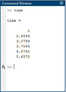
# min velocity of 3 rad/s and no acceleration limit. These
# are defined per-joint:
max_velocities = [3]
# No acceleration limits
max_accelerations = [np.inf]
# The minimum time between waypoints:
min_segment_time = 0.5

# Position waypoints
positions = [0, math.pi, 3, 2.5, 1, 0]

# Get times for each waypoint-to-waypoint segment:
segment_times = hebi.trajectory.estimate_segment_times(hebi.trajectory.TimeEstimationMethod.VelocityRamp, positions, max_velocities, max_accelerations, min_segment_time=min_segment_time)

# Create trajectory
waypoint_times = hebi.trajectory.segment_times_to_waypoints_times(segment_times)
trajectory = hebi.trajectory.create_trajectory(waypoint_times, positions);
If desired, you can also scale the trajectory, for example reducing to 80% of the speed:
trajectory = hebi.trajectory.create_trajectory(waypoint_times * 0.8, positions);Note that if you have explicit velocity or acceleration constraints passed into the create_trajectory function, you will also have to scale them appropriately (linearly for the velocity constraints and quadratically for the accelerations).
// min velocity of 3 rad/s and no acceleration limit. These
// are defined per-joint:
Eigen::VectorXd max_velocities(1);
max_velocities << 3;
// No acceleration limits
Eigen::VectorXd max_accelerations(1);
max_accelerations << std::numeric_limits<double>::quiet_NaN();
// The minimum time between waypoints:
double min_segment_time = 0.5;

// Position waypoints
Eigen::MatrixXd positions(1, 6);
positions << 0, M_PI, 3, 2.5, 1, 0;

// Get times for each waypoint-to-waypoint segment:
auto segment_times = hebi::trajectory::Trajectory::estimateSegmentTimesTrapezoidal(positions, max_velocities, max_accelerations, min_segment_time);

// Create trajectory
auto waypoint_times = hebi::trajectory::segmentTimesToWaypointsTimes(segment_times);
auto trajectory = hebi::trajectory::Trajectory::createUnconstrainedQp(waypoint_times, positions);
If desired, you can also scale the trajectory, for example reducing to 80% of the speed:
auto trajectory = hebi::trajectory::Trajectory::createUnconstrainedQp(waypoint_times * 0.8, positions);Note that if you have explicit velocity or acceleration constraints passed into the create_trajectory function, you will also have to scale them appropriately (linearly for the velocity constraints and quadratically for the accelerations).
Linear Movements
Minimum-jerk joint trajectories generate smooth human-like motion, but the end effector generally does not move linearly through space.
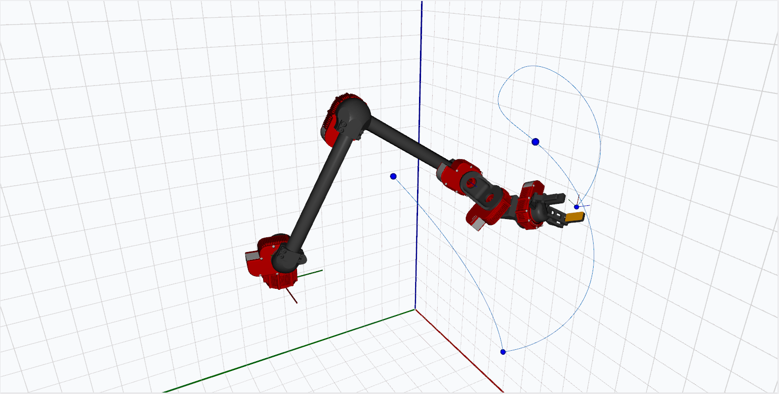
Linear cartesian motions can be generated by using inverse kinematics to sample desired joint positions along a linear path between the points. For example, interpolating the above joint motion in 25mm intervals yields the approximately linear motion below:
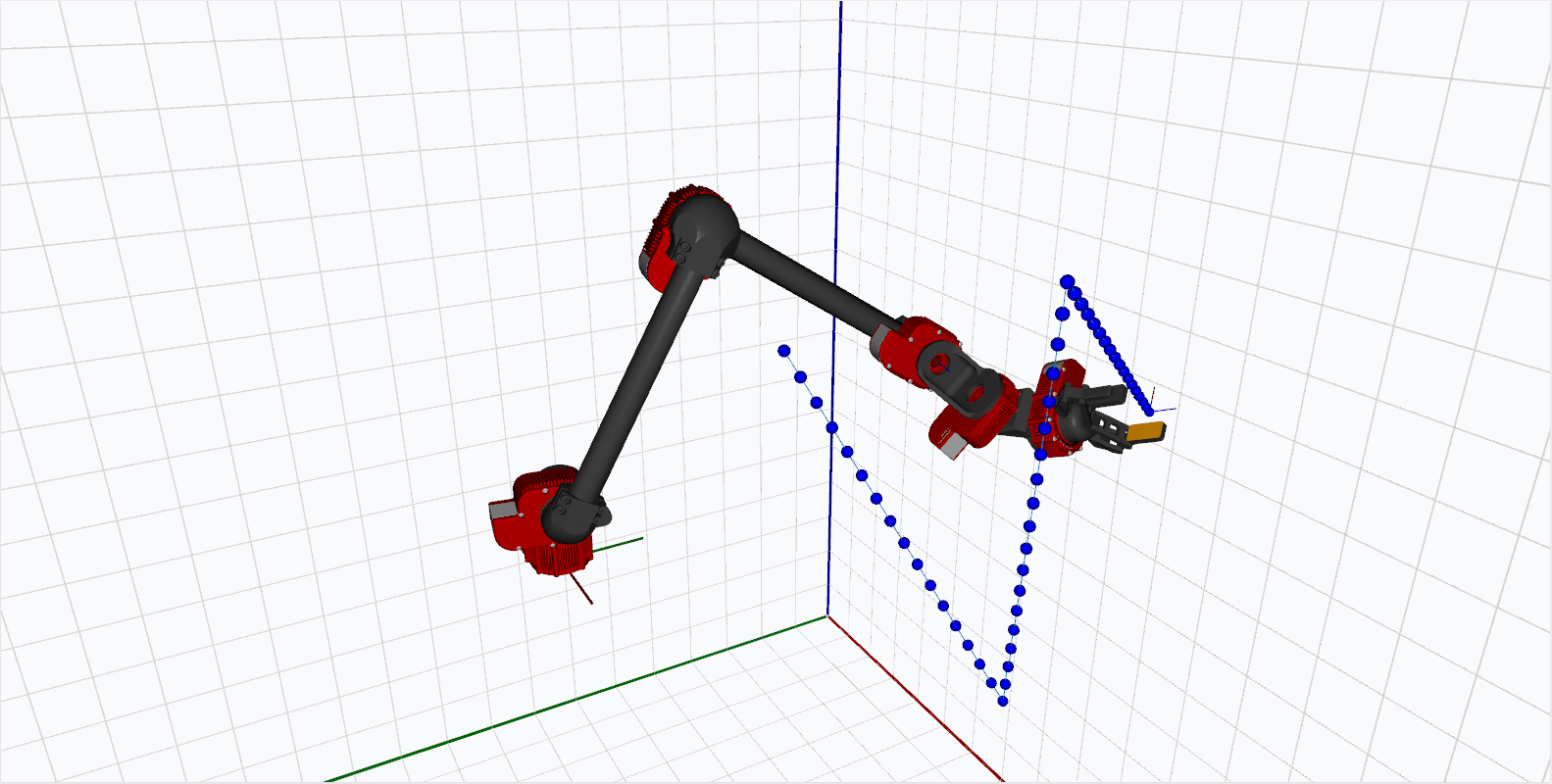
The details depend on the kinematic configuration and are typically application specific. In the MATLAB API, there is an included function newLinearMove that can serve as a starting point.
-
MATLAB
-
Python
-
C++
% Setup
kin = HebiUtils.loadHRDF('hrdf/A-2085-06G.hrdf');
trajGen = HebiTrajectoryGenerator(kin);

% Create joint waypoints
waypoints = [
    1.3958    1.0811    1.6582    7.6839    2.5466    9.4503
    1.0241    1.5928    1.4944    5.4796    3.0167    9.0366
];

% Compute linear trajectory w/ IK interpolations
trajectory = trajGen.newLinearMove(waypoints);
Not currently implemented in Python.
Not currently implemented in C++.
Arm API
The Arm API provides an abstraction for controlling a fixed base serial kinematic chain (e.g., a robot arm). Features include on-the-fly trajectory generation, built-in gravity and dynamics compensation, gripper support, and plugin features like impedance control. By coordinating joint commands, smooth trajectories to new positions, and kinematics calls, this results in less boilerplate user code while still allowing low-level access to the Group and Kinematics/RobotModel objects as needed.
Arm Creation
The config file format provides the necessary information to create an Arm object in the APIs. This includes the module names and families, corresponding HRDF file, gains, and other configuration information.
To create an Arm object from a config file, see the code snippets below:
-
MATLAB
-
Python
-
C++
Create a HebiArm from a config file:
config = HebiUtils.loadRobotConfig('my_robot.cfg.yaml');
arm = HebiArm.createFromConfig(config);
lookup = hebi.Lookup
config = hebi.config.load_config("my_robot.cfg.yaml")
arm = hebi.arm.create_from_config(config, lookup)std::vector<std::string> errors;
const auto config = hebi::RobotConfig::loadConfig("my_robot.cfg.yaml", errors);
if (config) {
auto arm = hebi::arm::Arm::create(*example_config);
}
Alternatively, you can create a HebiArm manually, by passing in a Group, Kinematics/RobotModel, and any desired plugin information directly.
|
Basic Usage
When using the Arm API, basic control of the robot can be achieved by calling update and send in a loop. The update call requests feedback, updates the state, and computes appropriate position, velocity, and torque (effort) commands. The commands can be modified by users before subsequently being sent out using the send function. This simple loop will maintain communication to the robot and, in absense of other commands, keep the system in a neutral "grav comp" configuration (assuming the grav comp plugin was enabled in the config file):
Basic control of the Arm involves setting a waypoint Goal. This is a set of joint positions (and optionally velocity and accelerations) at specific times relative to the current time. To do so, you call the "setGoal" command. Note that "setGoal" queues a smooth trajectory starting at the current state, and this motion continues as the "update" and "send" commands are run. For example, the code below will create and execute a smooth trajectory drive the robot to the "home" set of joint angles over 3 seconds, then will smoothly move to the "wait" set of joint angles over 3 seconds (and stay there until the program is killed). The outgoing commands include positions, velocities, and torques (efforts) to compensate for joint accelerations and gravity.
-
MATLAB
-
Python
-
C++
arm.update(); # Get initial data for the arm
arm.setGoal(home, 'time', 3);
while ~arm.isAtGoal
arm.update();
arm.send();
end
arm.setGoal(wait, 'time', 3);
while true
arm.update();
arm.send();
endarm.update() # Get initial data for the arm
goal = hebi.arm.Goal(arm.size)
goal.add_waypoint(t=3.0, position=home)
arm.set_goal(goal)
while not arm.at_goal():
arm.update()
arm.send()
goal = hebi.arm.Goal(arm.size)
goal.add_waypoint(t=3.0, position=wait)
arm.set_goal(goal)
while True:
arm.update()
arm.send()arm->update() # Get initial data for the arm
arm->setGoal(arm::Goal::createFromPosition(3, home));
while (!arm.atGoal()) {
arm->update():
arm->send()
}
arm->setGoal(arm::Goal::createFromPosition(3, wait));
while (true) {
  arm->update():
  arm->send()
}Arm Plugins
The Arm object also supports "plugins", which are run during the update and send calls. Plugins are called at the end of each update and may modify the state in arbitrary ways, such as modifying the commands sent to the arm. Two common examples are "gravity compensation" and "dynamics compensation" plugins, which provide additional effort commands to counteract gravity and add feed forward torques to accelerate the robot’s mass.
There are several built-in plugins we provide for abstracting commonly used functionality (see robot config plugin documentation), or users can inherit from the basic plugin classes and add their own plugins to the arm. Adding a plugin is done by adding to the plugin section of the robot config YAML file; see below for an example of the "plugins" section for each of the built-in plugins (full parameter documentation for each is at the link above):
If creating an arm manually without using a config file (not recommended), the gravity and dynamics compensation plugins are enabled by default for backwards compatibility with previous API versions. You can pass in parameters to the Arm constructor (Python/C++) or set the arm.plugins property (MATLAB, see HebiArmPlugin) to add other plugins.
|
-
The
GravityCompensationEffortplugin is recommended for most use cases, and adds torques to balance the estimated force of gravity. Note that due to inaccuracies in the torque sensor, this will not be exactly weightless and immobile for most systems, and the system may drift slightly.
- type: GravityCompensationEffort # "type" is the key used by API to identify each plugin
    # "name" is user friendly, and is available in APIs to
    # reference specific plugins (e.g., if you have multiple
    # of the same type)
    name: gravComp
    # Can be toggled in the API; this defines starting state.
    # Available for all plugins
enabled: true-
The
DynamicsCompensationEffortplugin is recommended for most use cases, and adds torques to balance the estimated force required to accelerate the masses of the robot as the joints accelerate. The masses are determined from the robot model, and the required torques are based on the current kinematic configuration and the corresponding Jacobian.
- type: DynamicsCompensationEffort
    name: dynamicsComp
    # When enabled or disabled, linearly scales contribution
    # of plugin over 5 seconds. Available for all plugins
ramp_time: 5-
The
EffortOffsetplugin can be used to add torque offsets for arms with gas springs. Around -7 Nm for most kits, but it may need to be tuned for your specific setup.
- type: EffortOffset
    name: gasSpringCompensation
offset: [0, -7, 0, 0, 0, 0]-
The
DoubledJointMirrorplugin takes actuator commands and splits them with a parallel actuator such as indouble-shoulderconfigurations. The naming convention for theDoubledJointplugin would be to add an "A/B" indication to the modules immediately after theJ#component.
- type: DoubledJoint
    group_family: J2B_shoulder
    group_name: Arm
    # 0-based index of joint to copy commands from
    index: 1
    # whether or not to mirror commands (depends on
    # robot configuration)
mirror: true-
The
ImpedanceControllerplugin adds impedance control on top of executing motions. For example, this configuration holds end effector position, but allows rotation around all axes.
- name: 'impedanceController'
    type: ImpedanceController
    gains_in_end_effector_frame: true
    kp: [500, 500, 500, 0, 0, 0]  # (N/m) or (Nm/rad)
    kd: [ 10,  10,  10, 0, 0, 0]  # (N/(m/sec)) or (Nm/(rad/sec))
To run the impendance controller, you often will clear (or de-weight the gains for) the position and velocity commands from the arm so the impendence efforts are the primary contributors to the system control:
-
MATLAB
-
Python
-
C++
% Disable position / velocity commands and run purely on gravity
% compensated impedance control
arm.setGoal(desiredPosition);
while true
    arm.update();
    arm.cmdPos = [];
    arm.cmdVel = [];
    arm.send();
end
import numpy as np
# Disable position / velocity commands and run purely on gravity
# compensated impedance control
arm.set_goal(desired_position);
while True:
arm.update()
arm.pending_command.position = [np.nan] * group.size
arm.pending_command.velocity = [np.nan] * group.size
arm.send()// Disable position / velocity commands and run purely on gravity
// compensated impedance control
arm->setGoal(arm::Goal::createFromPosition(desiredPosition));
while (true) {
arm->update();
for (int i = 0; i < group->size(); ++i) {
arm.pendingCommand[i].actuator().position().clear();
arm.pendingCommand[i].actuator().velocity().clear();
}
arm->send();
}More Info
The documentation here does not fully cover the features in the Arm API. More advanced behavior, such as modifying pending commands before they are sent to the arm, are demonstrated in various demo and example code. To get started, look in the "arms" section of the examples repositories for Matlab, python, and C++.
Mobile I/O API
For use cases that require user interaction we recommend exploring the Mobile I/O iOS and Android app. It provides joystick-like axes and buttons as well as a rich set of sensor inputs.
You can connect to a Mobile I/O application on the network by creating a Group directly (see group creation documentation), but we have provided convenience wrappers in the APIs to more naturally interface. These wrappers create a MobileIO object in code that allows you to set and receive state from the app. The API works similarly to the arm API in that the update call updates the internal state (axes, buttons, and sensor feedback).
Here is a simple example which prints out the orientation feedback (note — only available if AR support is turned on in the app!) until you press the b8 button:
-
MATLAB
-
Python
-
C++
In MATLAB the wrapper is the HebiMobileIO object:
% Block until the device is found on the network
mobileIO = HebiMobileIO.findDevice('HEBI', 'mobileIO');

% Continuously display orientation until button 8 gets pressed
while ~mobileIO.getFeedbackIO().b8
    mobileIO.update();
    disp(mobileIO.getOrientation());
end
In Python the wrapper is the MobileIO object.
# Can omit family and name to use these defaults as well
mobile_io = hebi.util.create_mobile_io(hebi.Lookup(), family='HEBI', name='mobileIO')
if mobile_io is None:
    print("Could not find mobile IO on network")
    return

# Continuously display orientation until button 8 gets pressed
while not mobile_io.get_button_state(8):
    mobile_io.update()
    print(mobile_io.orientation)
In C++ the wrapper is the hebi::util::MobileIO object.
// Can omit family and name to use these defaults as well
auto mobile_io = hebi::util::MobileIO::create("HEBI", "mobileIO");
if (!mobile_io) {
    std::cout << "Could not find mobile IO on network\n";
    return;
}

// Continuously display orientation until button 8 gets pressed
while (!mobile_io.getButton(8)) {
    mobile_io->update();
    auto orient = mobile_io->getArOrientation();
    std::cout << "[" << orient.getW() << ", " << orient.getX() << ", " << orient.getY() << ", " << orient.getZ() << "]\n";
}
Devices that are connected using wireless networks can occasionally experience latency spikes or dropped packets. The default behavior of the update function of the MobileIO class is to block until a defined timeout while waiting for incoming packets. In cases where the app is used to control a robot, it is typically desirable to never block the control loop and to update the target only when there is new information.
One method to handle this is to use a separate thread to handle events from the mobile IO device, then parse and place into an event queue that is read from the control thread.
Another approach is to use a non-blocking overload for the update function.
-
MATLAB
-
Python
-
C++
% Block until the device is found on the network
mobileIO = HebiMobileIO.findDevice('HEBI', 'mobileIO');
quitDemoButton = 'b8'; % overload for more readable access

% Display updated feedback only when available
while ~mobileIO.getFeedbackIO().(quitDemoButton)

    % Try to update mobileIO
    [hasNewFeedback, timeSinceLastFeedback] = mobileIO.update('timeout', 0);
    if hasNewFeedback
        disp(mobileIO.getOrientation());
    elseif timeSinceLastFeedback > 3
        error('We have not received mobileIO feedback for 3 seconds!');
    end

    % Do robot control (placeholder here)
    arm.update();
    arm.send();

end
QUIT = 8
mobile_io = hebi.util.create_mobile_io(hebi.Lookup(), family='HEBI', name='mobileIO')
if mobile_io is None:
print("Could not find mobile IO on network")
return
# Display updated feedback only when available
while not mobile_io.get_button_state(QUIT):
# Try to update mobileIO
got_feedback = mobile_io.update(timeout_ms=0)
if got_feedback:
print(mobile_io.orientation)
# Do robot control (placeholder here)
arm.update()
arm.send()const int QUIT = 8;
auto mobile_io = hebi::util::MobileIO::create("HEBI", "mobileIO");
if (!mobile_io) {
std::cout << "Could not find mobile IO on network\n";
return;
}
// Display updated feedback only when available
while (!mobile_io.getButton(QUIT)) {
// Try to update mobileIO
bool got_feedback = mobile_io->update(0);
if (got_feedback) {
auto orient = mobile_io->getArOrientation();
std::cout << "[" << orient.getW() << ", " << orient.getX() << ", " << orient.getY() << ", " << orient.getZ() << "]\n";
}
// Do robot control (placeholder here)
arm->update()
arm->send()
}Accessing Mobile IO State
The MobileIO class contains various states that are updated when update is called, including inertia sensors, temperature, and various components of the normal feedback objects. These can generally be accessed by calling getLastFeedback() after calling update:
-
MATLAB
-
Python
-
C++
gyro = mobileIO.getFeedback().gyrogyro = mobile_io.get_last_feedback().gyroconst hebi::Feedback& last_feedback = mobile_io->getLastFeedback();
auto gyro_feedback = last_feedback.imu().gyro().get();Additionally, however, there are a few states unique to the MobileIO app:
-
AR (Augmented Reality) Orientation and Position: These are relatively accurate 3D pose estimates provided by ARkit (on iOS) and ARCore (on Android). Note that they can be disabled to save battery in the Mobile IO app, and so will not always be populated in the returned feedback
-
Button State: The buttons in the Mobile IO default layout are mapped to the B-channel IO pins in the underlying feedback object. However, they are exposed in the
MobileIOwrapper directly, including (in C++ and Python) functions to get the difference between the last feedback received and the feedback before that (useful for helping to detect edge triggers without additional bookkeeping in the code). -
Axis State: The axes in the Mobile IO default layout are mapped to the A-channel IO pins in the underlying feedback object. Like the buttons, they are exposed directly in the
MobileIOwrapper.
-
MATLAB
-
Python
-
C++
ar_orientation = mobileIO.getArOrientation()
ar_pose = mobileIO.getArPose()

% Get buttons and axes from "IO Feedback"
axis_1_value = mobileIO.getFeedbackIO().a1
button_8_value = mobileIO.getFeedbackIO().b8

% Note there is no "ButtonDiff" helper function in
% MATLAB; instead you can track and compare with
% previous state
was_button_3_pressed = button_3_value == 1 && prev_button_3_value == 0
ar_position = mobile_io.position
ar_orientation = mobile_io.orientation
axis_1_value = mobile_io.get_axis_state(1)
button_8_value = mobile_io.get_button_state(8)
# -1 is "ToOff", 0 is "Unchanged", 1 is "ToOn"
button_3_change = mobile_io.getButtonDiff(3)
was_button_3_pressed = (button_3_change == 1)hebi::Vector3f ar_position = mobile_io->getArPosition();
hebi::Quaternionf ar_orientation = mobile_io->getArOrientation();
float axis_1_value = mobile_io->getAxis(1);
float button_8_value = mobile_io->getButton(8);
bool was_button_3_pressed = (mobile_io->getButtonDiff(3) == ButtonState::ToOn);App Layout Setup
HebiMobileIO also provides a way to setup the user interface as shown below. We recommend using layout JSON files (see the arm layout examples, as well as the corresponding usages in the Matlab, python, and C++ example repos).
-
MATLAB
-
Python
-
C++
Please refer to the HebiMobileIO docs for more detailed information.
% Setup mobileIO UI
mobileIO = HebiMobileIO.findDevice('HEBI', 'mobileIO');
mobileIO.initializeUI();
mobileIO.sendLayout("path/to/layout.json");
mobile_io = hebi.util.create_mobile_io(hebi.Lookup())
mobile_io.resetUI()
success = mobile_io.send_layout(layout_file='path/to/layout.json')auto mobile_io = hebi::util::MobileIO::create("HEBI", "mobileIO");
mobile_io->resetUI();
bool success = mobile_io->sendLayout("path/to/layout.json");The layout can also be configured manually in code by individually addressing elements:
-
MATLAB
-
Python
-
C++
% Setup mobileIO UI
mobileIO = HebiMobileIO.findDevice('HEBI', 'mobileIO');
mobileIO.initializeUI();
mobileIO.setAxisValue([3 6], [-1 1]);
mobileIO.setButtonIndicator([1 8], true);
mobileIO.addText('B1 - Reset/re-align pose');
mobileIO.addText('A3 - Scale translation commands');
mobileIO.addText('A6 - Gripper Open/Close');
mobileIO.addText('B8 - Quit');
# Setup mobileIO UI
mobile_io = hebi.util.create_mobile_io(hebi.Lookup())
mobile_io.resetUI()
mobile_io.set_axis_value(3, -1)
mobile_io.set_axis_value(6, 1)
mobile_io.set_button_output(1, 1)
mobile_io.set_button_output(8, 1)
mobile_io.add_text('B1 - Reset/re-align pose')
mobile_io.add_text('A3 - Scale translation commands')
mobile_io.add_text('A6 - Gripper Open/Close')
mobile_io.add_text('B8 - Quit')// Setup mobileIO UI
auto mobile_io = hebi::util::MobileIO::create("HEBI", "mobileIO");
mobile_io->resetUI()
mobile_io->setAxisValue(3, -1);
mobile_io->setAxisValue(6, 1);
mobile_io->setButtonLed(1, 1);
mobile_io->setButtonLed(8, 1);
mobile_io->appendText('B1 - Reset/re-align pose');
mobile_io->appendText('A3 - Scale translation commands');
mobile_io->appendText('A6 - Gripper Open/Close');
mobile_io->appendText('B8 - Quit');Logging
Data logging, visualization, and analysis tools are a critical part of robotics development. We provide powerful logging capabilities that allow the logging of data in excess of 1kHz, from any number of devices, and over extended periods of time (multiple days). Logging is done in the background (e.g., in MATLAB entirely outside of the main thread), and written directly to disk so that there is no performance impact on real-time control logic. This also means that in case the program ever crashes due to unforeseen circumstances, none of the logged data is ever lost.
The logging format is also common across all HEBI APIs, so logs saved with by one API can read by any of the other APIs.
Here is a simple example of logging data; the logging occurs at the group’s feedback frequency:
-
MATLAB
-
Python
-
C++
% Log data for 5 seconds
group.startLog();
pause(5);
data = group.stopLog();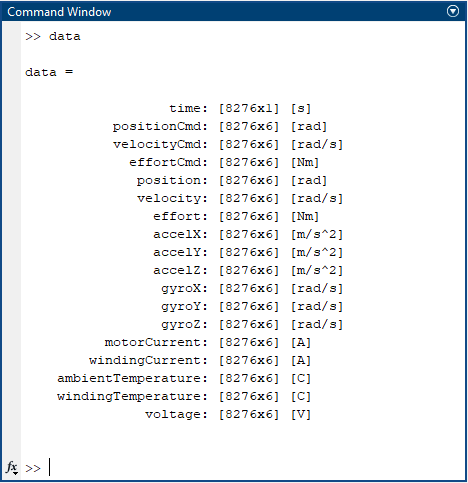
# get "group" from lookup
...

# Start logging (note that extension is needed)
log_file_location = group.start_log('/path/to/output', 'filename.hebilog')

# main control logic here
...

# Stop logging
group.stop_log()
Additionally, you can optionally provide the directory and/or file name for the log file like:
# Will start a log in the process' current working directory, with
# a name generated using the timestamp of the current time and date
log_file_location1 = group.start_log()

# Will generate a name in the provided directory
log_file_location2 = group.start_log(directory='/path/to/output')
The log data is stored in a file on disk. The name is returned with the initial Group.start_log call, and is also retrievable through the LogFile object returned when stopping the log.
// get hebi::Group "group" from lookup
...

// Start logging (can also specify log file name as second parameter)
std::string full_log_path = group->startLog("./test_logs/");

// main control logic here
...

// Stop logging
std::shared_ptr<hebi::LogFile> log_file = group->stopLog();
The log data is stored in a file on disk; the name is returned with the initial "startLog" call, and is also retrievable through the LogFile object returned when stopping the log.
Note that if the "stopLog" call returns an empty shared_ptr object, this indicates that the call failed and the log file was not created; this is usually caused by there being no active log that has been started.
Reading Logs
The return value of "stop log" returns a log object that can be used for accessing the data within the log.
-
MATLAB
-
Python
-
C++
The fields of the object returned from stopLog can be accessed directly, as with the returned feedback from getNextFeedback.
Note that as with getting feedback from a group, there are variants for stopLogFull, stopLogIO, and stopLogMobile to return different views of the data.
% Read the position and position command from the log
data = group.stopLog();
pos_fbk = data.position;
pos_cmd = data.positionCmd;| The default stopLog call returns a Java object that contains all the data. Thus, each access needs to convert the underlying Java type to the corresponding MATLAB type. This is typically not an issue, but if you need to access fields many times, we recommend converting the Java object to a MATLAB struct via struct(data). |
The returned LogFile object allows sequential access to the content in the log file. The below example demonstrates analysing a logfile to find the highest torque experienced by each joint:
num_modules = log_file.number_of_modules
feedback = hebi.GroupFeedback(num_modules)

# If we are trying to find the max, start with the lowest possible number.
max_efforts = np.array([-np.inf] * num_modules, dtype=np.float64)

# Reuse feedback as a best practice
feedback = log_file.get_next_feedback(feedback)
# Get the component-wise max each feedback entry compared to the running max efforts
while feedback is not None:
  max_efforts = np.maximum(max_efforts, feedback.position)
  feedback = log_file.get_next_feedback(feedback)
The returned LogFile object (see API reference documentation) allows sequential access to the content in the log file; the below example demonstrates analysing a logfile to find the highest torque experienced by each joint:
size_t num_modules = log_file->size();
GroupFeedback feedback(num_modules);
Eigen::VectorXd max_efforts(num_modules);
// If we are trying to find the max, start with the lowest possible number.
max_efforts::setConstant(-std::numeric_limits<double>::infinity());

// Get the component-wise max each feedback entry compared to the running max efforts
while (log_file->getNextFeedback(feedback))
  max_efforts = max_efforts.cwiseMax(feedback.getPositions());
Loading logs from file
The log object returned from "stop log" can also be returned from a previously saved log (written by any API).
-
MATLAB
-
Python
-
C++
All logging happens in the background and gets stored on disk in a binary streaming format. The default stopLog() call converts the binary format into another format that MATLAB can work with. We also provide the convertGroupLog() utility to load raw log files that were previously saved or generated using other APIs.
% load raw log file
binaryFile = '2015-12-02_17-02-12.994887.hebilog';
matFile = HebiUtils.convertGroupLog(binaryFile, 'format', 'mat', 'view', 'full');
data = load(matFile);
Replaying Logs
We also added the newGroupFromLog utility which supports replaying log files via the standard group interface. After loading the log, each call to getNextFeedback on the group returns the next feedback in sequence (including the logged timestamp), regardless of the rate it is actually being called. This is useful, for example, for online algorithm development while working with offline data.
% Iteratively step through log file
group = HebiUtils.newGroupFromLog(path);
while true
    fbk = group.getNextFeedback();
    disp(fbk.position);
end
You can manually create a LogFile object from an existing file:
import hebi
log_file = hebi.util.load_log('/path/to/file.hebilog')
You can manually create a LogFile object from an existing file using:
std::shared_ptr<hebi::LogFile> log_file = hebi::LogFile::open("/path/to/file.hebilog");Visualizing logs
-
MATLAB
-
Python
-
C++
Logs are returned as structures where data is organized in vectors and matrices so that the resulting data interacts well with MATLAB’s built-in plotting tools.
% Plot logged data and overlay commanded and feedback position
figure(); hold on;
plot(data.time, data.position);
plot(data.time, data.positionCmd, ':');
Additionally, we provide HebiUtils.plotLogs to help with basic feedback plots.
% Plot position (can be any field available in the log)
HebiUtils.plotLogs(data, 'position')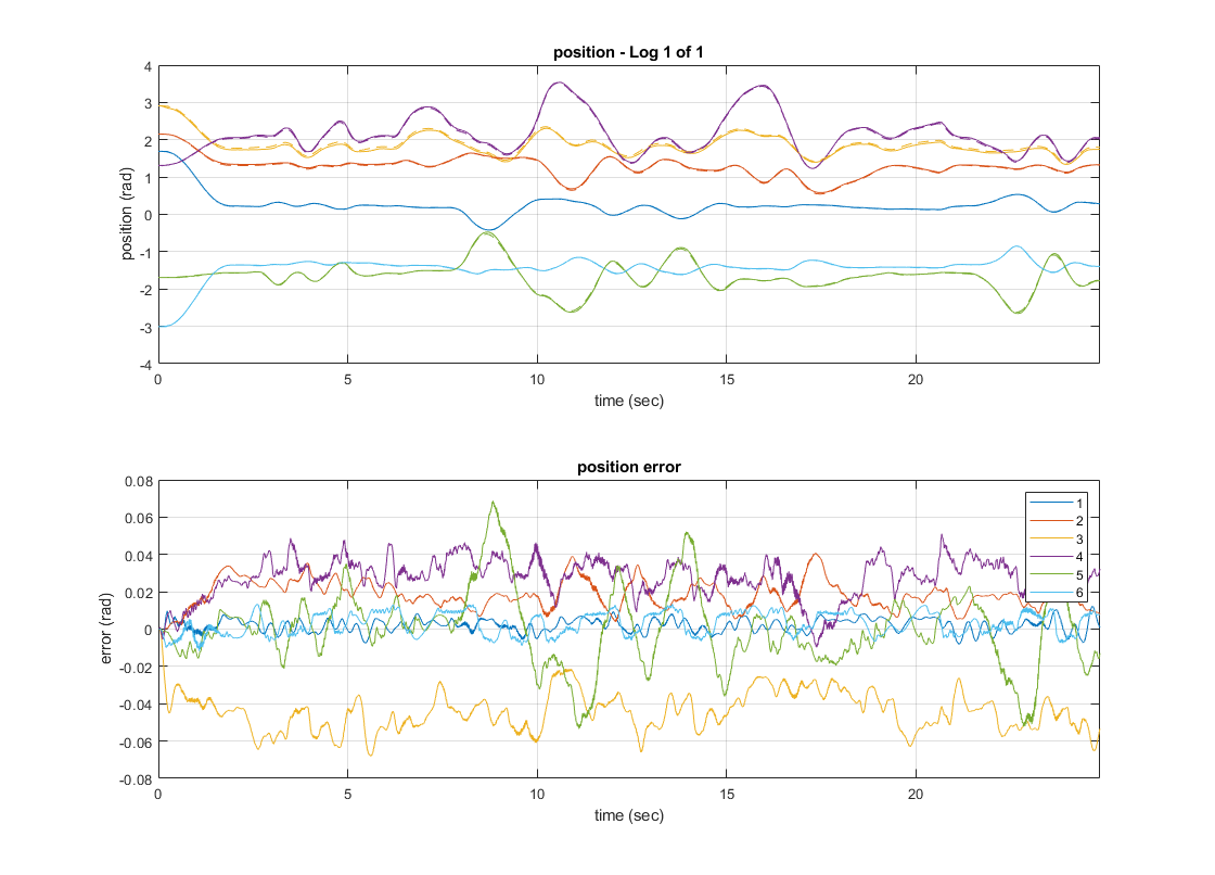
Currently to visualize data from logs, you must use a charting library. More examples will be provided soon!
You must use a charting library to visualize data from the logs. Examples in the [C++ examples repo contain several examples of using the beta hebi-charts library to provide this functionality. The following shows saving position feedback from a log into a vector and plotting it; it was taken from the position command example:
// Plot the logged position data
std::vector<std::vector<double>> pos;
pos.resize(group->size());
// Track time offset so times[0] = 0 at the end for plotting convenience
double t0{};
std::vector<double> times;
GroupFeedback fbk(group->size());
// Iterate through the logs to read each feedback sequentially
while(log_file->getNextFeedback(fbk)) {
  for(size_t i = 0; i < group->size(); i++){
    pos[i].push_back(fbk.getPosition()[i]);
  }
  if (t0 == 0)
    t0 = fbk.getTime();
  times.push_back(fbk.getTime() - t0);
}

// Visualize data
hebi::charts::GridWindow window;
auto chart = window.addLineChart();
for(size_t i = 0; i < group->size(); i++){
  auto title = (std::string("module ") + std::to_string(i));
  chart.addLine(title, times, pos[i]);
}
window.show();

hebi::charts::framework::waitUntilWindowsClosed();
Logging over extended periods of time
To avoid very large files from a long-running process, you can split logs into e.g. 1 hour chunks. This also allow for incremental uploading of the finished logs to a server, for example.
-
MATLAB
-
Python
-
C++
The conversion run when calling stopLog would be too expensive to do inside a loop, so instead we can call startLog to finish the previous log and to start a new one. The startLog command is comparatively very cheap and may be called inside a tight loop.
% log continously over an extended period of time
binaryFiles = {};
t0 = tic();
while true

    % run control loop
    % ...

    % create a new log every hour
    if toc(t0) > 3600
        binaryFiles{end+1} = group.startLog();
        t0 = tic();
    end

end
The resulting log files can then be loaded once a task is done, or from a different MATLAB instance while the task is still running.
% convert log files offline
nFiles = length(binaryFiles);
for i = 1:nFiles
    disp(['converting log ' num2str(i) '/' num2str(nFiles)];
    matFile = HebiUtils.convertGroupLog(binaryFile, 'format', 'mat', 'view', 'full');
end
Currently, the startLog function in Python adds a delay while retrieving information from the Group, and so cannot be used as described for MATLAB here. The best approach in Python is to handle the log start/stop in a background thread.
Currently, the startLog function in C++ adds a delay while retrieving information from the Group, and so cannot be used as described for MATLAB here. The best approach in Python is to handle the log start/stop in a background thread.
ROS 2 API
| The ROS documentation is primarily maintained at https://github.com/HebiRobotics/hebi_ros2_examples |
Overview
To make it convenient to use ROS with HEBI products, we have created a set of nodes and full system examples to allow you to interface with HEBI systems. These examples include using ROS to control a HEBI arm, mobile bases, integration with MoveIt!, Gazebo simulation integration, and Rviz visualization. These are documented at https://github.com/HebiRobotics/hebi_ros2_examples.
We also provide a library of XACRO macros in the hebi_description package to help you build up systems from HEBI components quickly. Additionally, the package includes a script for converting HRDF files to URDF, for easier setup.
Internally, the ROS 2 APIs and examples use the HEBI C++ API to connect to HEBI components. For those wishing for more flexibility or to develop custom nodes, we have created a ROS 2 package that wraps the HEBI C++ API (https://github.com/HebiRobotics/hebi_cpp_api_ros/). This can be installed as a package on humble, iron or jazzy using apt install ros-<distro>-hebi-cpp-api. For use of the C++ API in ROS, the examples shown above provide a good starting point; further documentation is available in the HEBI APIs overview.
ROS 1 (Legacy)
The HEBI ROS 1 packages are no longer being actively maintained, and we highly recommend anyone still using this to transition to ROS 2 packages. Please email support@hebirobotics.com for assistance in this process!
|
The ROS 1 documentation is available at wiki.ros.org, in particular at http://wiki.ros.org/hebi_cpp_api_examples and http://wiki.ros.org/hebi_cpp_api
Other approaches
Python It is also possible to call the HEBI Python API directly in your node; we do not currently have public examples for this approach.
File Formats
Robot Config
The Robot Config file is a YAML-based format designed to store configuration information about a full system in a human-readable cross-API format.
The complete format, including past versions and example files using this format, is documented at https://github.com/HebiRobotics/robot-config.
Briefly, the format consists of a series of YAML elements that provide information about the used actuators, gains, kinematic structure, and optional plugins. For example, this snippet shows the robot config for a 6-DOF arm kit:
# X-Series 6-DoF Arm
version: 1.0
families: ["Arm"]
names: ["J1_base", "J2_shoulder", "J3_elbow", "J4_wrist1", "J5_wrist2", "J6_wrist3"]
hrdf: "../hrdf/A-2085-06.hrdf"

gains:
    default: "../gains/A-2085-06.xml"

user_data:
    # Default seed positions for doing inverse kinematics
    ik_seed_pos: [0.01, 1.0, 2.5, 1.5, -1.5, 0.01]

plugins:

  - type: GravityCompensationEffort
    name: gravComp
    enabled: true
    ramp_time: 2

  - type: DynamicsCompensationEffort
    name: dynamicsComp
    enabled: true
    ramp_time: 2
HRDF
The HEBI Robot Description Format (HRDF) is an XML-based format that allows kinematics and dynamics information about a robot configuration to be stored as a file that can be used by a variety of tools.
The complete format, including past versions and example files using this format, is documented at http://github.com/HebiRobotics/hebi-hrdf/.
Briefly, the format consists of a series of XML elements which define a kinematic chain of components. For example, this snippet shows the HRDF for a 5-DOF arm kit:
<robot>
<actuator type="X8-9"/>
<bracket type="X5HeavyRightOutside"/>
<actuator type="X8-16"/>
<link type="X5" extension="0.325" twist="3.141593"/>
<actuator type="X8-9"/>
<link type="X5" extension="0.325" twist="3.141593"/>
<actuator type="X5-1"/>
<bracket type="X5LightRight"/>
<actuator type="X5-1"/>
</robot>This format supports standard HEBI components, as well as generic rigid bodies and massless joints. As new components are added or new features supported by the URDF format, the version number of the format is incremented increased. Each API version explicitly supports a given version of the format.
Version 1.0.0 of the format supports the following elements. Note the attributes correspond to the documented parameters of the HEBI components.
| Element | Attribute | Description | Values |
|---|---|---|---|
|
|
The type of HEBI actuator module |
|
|
|
The type of HEBI link |
|
|
The length of the link, from center point to center point of mounting brackets (in meters) |
Floating point value |
|
|
The rotation about the extension axis (tube) of the link (in radians) |
Floating point value |
|
|
|
The type of HEBI bracket module |
|
|
|
The mass of the body (in kilograms) |
Floating point value |
|
The rotation matrix describing the orientation of the center of mass relative to the input. This is used for simplifying the inertia tensor description if desired. |
space-delimited, row-major 3x3 matrix of floating point values, |
|
|
The x-y-z position of the center of mass relative to the input (defaults to [0,0,0]) |
Space-delimited, 3-element vector of floating point values |
|
|
The rotation matrix describing the orientation of the output frame relative to the input frame, expressed in the input frame. (Defaults to 3x3 identity matrix) |
Space-delimited, row-major 3x3 matrix of floating point values |
|
|
The x-y-z position of the output frame relative to the input, expressed in the input frame. (defaults to [0,0,0]) |
Space-delimited 3-element vector of floating point values |
|
|
The moments of inertia, expressed in the center-of-mass frame. (each inertia moment defaults to 0) |
Floating point value |
|
|
|
The rotational or translational degree of freedom about a principal coordinate axis. |
|
XML Gains Format
In addition to direct programmatic access to setting controller gains, gains can also be stored in a XML file format that is universal to the HEBI APIs and Scope. This format allows gains to be loaded from a file and sent to a group of modules, or saved from a group of modules to a file.
| Saving the gains from a module or group of modules will capture all of the settable parameters, including the control strategy. |
The format is series of XML elements whose content is a list of values for each module in the group. For example, this snippet shows position PID gains for a set of 3 modules:
<?xml version="1.0" encoding="UTF-8" standalone="no"?>
<group_gains>
<control_strategy>3 3 3</control_strategy>
<position>
<kp>1 1.2 3</kp>
<ki>0 0 1.1</ki>
<kd>0 0.0001 0.001</kd>
</position>
</group_gains>This format supports all available gains for the position, velocity, and effort controllers, as can be seen in our downloadable default gains.
Saving and Loading Gains
Scope, as well as the C, C++, Python, and MATLAB APIs all have tools to read and write this gain format.
| Note that in each case below the gains will be set on the module, but not "persisted" to internal memory so that they apply on the next reboot of the module. Remember to 'persist' these gains if desired! |
In the Scope GUI, the currently active gains can be saved to a file by using the "Save to File" button on the "Gains" tab, and the gains in a file can be written to a module by using the "Load File" button. The "Load Defaults" button loads the default gains for the selected module and control strategy. Differences between the input fields and the currently set values will be highlighted.
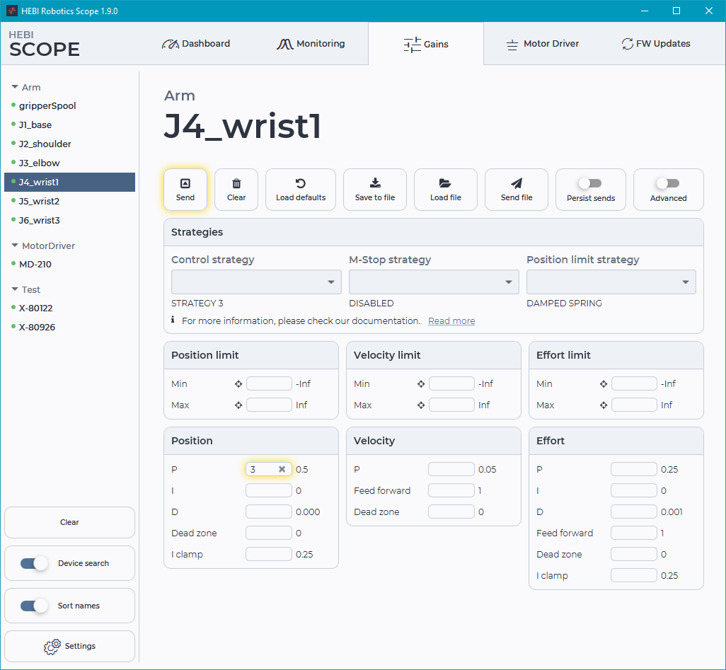
In the MATLAB API, these gains can be saved and loaded using function in the HebiUtils class:
% Saving gains from a group of modules
gains = group.getGains()
gainFile = HebiUtils.saveGains(gains, 'MyGains');
% Loading XML file gains and setting on group of modules
gains = HebiUtils.loadGains(gainFile);
group.send('gains', gains);In the C++ API, these gains can be saved and loaded by using the following code, assuming you have created a Group (see Gains API documentation for more info).
// Saving gains from a group of modules:
GroupInfo group_info(group->size());
if (group->requestInfo(&group_info))
group_info.writeGains("saved_gains.xml");
// Loading gains from a file onto a group of modules:
GroupCommand group_cmd(group->size());
group_cmd.readGains("saved_gains.xml");
bool success = group->sendCommandWithAcknowledgement(group_cmd);XML Safety Parameters
In addition to direct programmatic and UI access to setting safety parameters such as position limits, m-stop strategies, etc, these can also be stored in a XML file format that is universal to the HEBI APIs and Scope.
This format allows safety parameter to be loaded from a file and sent to a group of modules, or saved from a group of modules to a file.
The format is series of XML elements whose content is a list of values for each module in the group. For example, this snippet shows position limits and posiiton limit strategies for a set of 4 modules:
<?xml version="1.0" encoding="UTF-8" standalone="no"?>
<group_safety version="1.0.0">
<mstop>
<strategy>motor_off motor_hold disabled motor_off</strategy>
</mstop>
<position>
<limit_strategy>motor_hold motor_off disabled spring</limit_strategy>
<min_limit>-1.5 0 -inf -inf</min_limit>
<max_limit>1.5 1 inf inf</max_limit>
</position>
</group_safety>This format is fully documented here.
Saving and Loading Safety Parameters
The MATLAB API is currently the only API supporting reading and writing this format.
| Note that in each case below the parameters will be set on the module, but not "persisted" to internal memory so that they apply on the next reboot of the module. Remember to 'persist' these gains if desired! |
In the MATLAB API, these params can be saved and loaded using function in the HebiUtils class:
% Example (Saving gains to XML file)
safetyParams = group.getSafetyParams();
HebiUtils.saveSafetyParams(safetyParams, 'mySafetyParams.xml');
% Example (Loading gains from XML file and setting on a group):
safetyParams = HebiUtils.loadSafetyParams('mySafetyParams.xml');
group.send('SafetyParams', safetyParams);In the Python and C++ APIs, these gains can be saved and loaded through the Group object (see safety parameters documentation for more info).
XML Motor Driver Format
Motor driver configurations are stored in an XML format and can be loaded/sent from Scope or the hebi-config CLI. Each file specifies the configuration for one motor driver. For example, you can send files from the CLI with the following command,
hebi-config --name MD-210 --motor-driver-xml <file.xml> --persist --reset
The configuration is quite extensive and difficult to write from scratch. The easiest way to generate a file is to use Scope for the initial configuration and then click Save to file.
A small sample is in the snippet below. Note that you can use <xi:include> tags to share common configurations.
<?xml version="1.0"?>
<motor_driver_config xmlns:xi="http://www.w3.org/2001/XInclude">
<xi:include href="configs/motors/EC90_220W.xml" parse="xml" />
<xi:include href="configs/boards/SPI_80A_10VV.xml" parse="xml" />
<driver_calibration>
<winding_order value='ABC'/>
<hall_order value='ABC'/>
</driver_calibration>
<control_config>
<mode value='FOC_TORQUE_CONTROL'/>
<foc_gains>
<kp value='0.756'/>
<ki value='0.0717'/>
<i_clamp value='5'/>
</foc_gains>
<overmodulation value='1.15'/>
<hall_config>
<direction value='FORWARD'/>
<velocity_filter_size value='1'/>
</hall_config>
<encoder_a2_config>
<direction value='FORWARD'/>
<velocity_filter_size value='10'/>
</encoder_a2_config>
<motor_encoder_selection value='A2'/>
</control_config>
<drivetrain_config>
<gear_efficiency value='1'/>
<gear_ratio value='1'/>
</drivetrain_config>
</motor_driver_config>You can find more complete examples in BLDC_EC-Flat60_24V_150W_CONFIG.xml and FOC_EC-Flat90_24V_220W_CONFIG.xml.
The full schema is described in motor_driver_schema.xml.
API Best Practices
Naming Conventions
In order to have consistency across systems, apps, apis, and example code HEBI Robotics uses a standard convention for naming hardware that makes use of simple letter and number combinations. All HEBI products follow these conventions when shipped, and we encourage all our users to use it as well.
Family Names
Families help to group modules together. Doing so correctly is especially useful and important when you have multiple robots connected to a network at the same time. Check our documentation on Groups to learn more.
All actuators involved in a given kit (Igor, Hexapod, etc.) should be assigned the same Family. As such, the Family assigned should represent the name of that kit.
For example, all actuators in an X-Series Hexapod kit would be have the family Daisy.
Remember to include all modules involved with the kit. Don’t forget mobileIO and gripperSpool!
|
By convention, Family names should:
-
Be uppercase (i.e.
Rosie) -
Use your actuator model for single actuators (i.e.
X8-16) -
Use
IO_basicfor IO boards
Actuator Names
Our actuators look the same but can be used in multiple different ways; using our conventions can save you time and effort in identifying and debugging the right actuator.
Actuators in Serial Configuration
J#_<type>
Here, J# indicates where the actuator exists along the chain (it is the #th actuator in the chain) and <type> describes what the actuator is acting as. For example J2_shoulder would be the second actuator in the serial chain and the shoulder joint in an arm.
Thus, the standard naming for a 6-DoF arm:
J1_base, J2_shoulder, J3_elbow, J4_wrist1, J5_wrist2, J6_wrist3
If there is only one wrist actuator, like in a 4-DoF arm kit, remove the trailing number: J4_wrist
|
Special Conditions for Arms
-
If you have 2 or more elbows:
J3_elbow1,J3_elbow2, etc… -
If you have 2 actuators in parallel:
J2A_shoulder,J2B_shoulder-
A is the one the HRDF follows through.
-
The HRDF will typically follow the left side (relative to the base module). Hence, the convention follows as Left = A and Right = B, but ALWAYS double check with the HRDF.
-
-
The 2 rules above can combine:
J2A_shoulder1,J2B_shoulder1,J3_shoulder2, and so on.
Grippers
If your kit makes use of a standard HEBI parallel gripper, you will have a spool actuator that you command to change the state of the gripper. As per our convention, this actuator is named gripperSpool.
Mobile Base Wheels
-
Omni-base:
W1,W2,W3(refer to Omni-Base Reference Drawing) -
Diff Drive Base:
W1_left,W2_right -
Mecanum Base:
W1_frontLeft,W2_backLeft,W3_frontRight,W4_backRight
Multi-limbed Robots
L#_J#_<function>
Here, L# indicates which limb we are looking at. Each standard robot kit created by HEBI Robotics has a predefined layout of limb numbers that can be found on that kit’s reference documentation.
Here is an example of how the "Daisy" Hexapod kit is named (see page 31 of Hexapod Manual for leg layout):
L1_J1_base, L1_J2_shoulder, L1_J3_elbow, L2_J1_base, L2_J2_shoulder, L2_J3_elbow, etc…
Special Condition: Igor
For the Igor kit the arms and legs have been named in the following fashion:
-
Left = 1 and Right = 2 (Igor Manual)
-
Legs:
L1_J3_wheel, L2_J3_wheel, L1_J1_hip, L1_J2_knee, L2_J1_hip, L2_J2_knee -
Arms:
A1_J1_base, A1_J2_shoulder, A1_J3_elbow, A1_J4_wrist, A2_J1_base, A2_J2_shoulder, A2_J3_elbow, A2_J4_wrist
Mobile devices
If you are using your mobile device to provide input to your program, your device should be named mobileIO. This can be set in the settings on your phone, or using Scope.
Single Actuators
Use the actuator’s serial number. For example: X-00542. This number is printed on the actuator, or can be seen on Scope.
IO Boards
Use the board’s serial number. For example: IO_00042. This number is printed on the board, or can be seen on Scope.
| Note that IO board serial numbers use underscores instead of hyphens. |
Arm Kit Numbering
Our arm kits are numbered to make it faster for you to identify one arm from another. By looking only at an arm kit number, you should be able to discern which type (X-series or R-series) of actuators your arm is made of, the degrees of freedom in you arm, and the addition of any add-ons, such as a gripper, to your configuration. We use this numbering to name our kinematic (.hrdf) and gains (.xml) files.
Grippers are included in the HRDF file, but not the gains file. For example, in the case of a 6-dof x-series arm with a gripper, the HRDF will be named A-2085-06G.hrdf, but the gains file will be A-2085-06.xml.
|
Learn more about our arm kits at our Kit documentation or our Arms page.
| Arm Kit Number | Description |
|---|---|
|
X-Series arm kit with |
|
X-Series arm kit with an X-Series gripper as the end effector. |
|
R-Series arm kit with |
|
R-Series arm kit with an R-Series gripper as the end effector. |
Special Cases
| Arm Kit Number | Description |
|---|---|
|
X-Series SCARA style arm with 4 degrees of freedom. |
|
X-Series double shoulder arm kit with 7 degrees of freedom. |
|
R-Series SCARA style arm with 4 degrees of freedom. |
|
R-Series double shoulder arm kit with 7 degrees of freedom. |